Linear Algebra and Linear Regression

Review

• Last time: Looked at objective functions for movie recommendation.
• Minimized sum of squares objective by steepest descent and stochastic gradients.
• This time: explore least squares for regression.

Regression Examples

• Predict a real value, \(\dataScalar_i\) given some inputs \(\inputVector_i\).
• Predict quality of meat given spectral measurements (Tecator data).
• Radiocarbon dating, the C14 calibration curve: predict age given quantity of C14 isotope.
• Predict quality of different Go or Backgammon moves given expert rated training data.

Olympic 100m Data

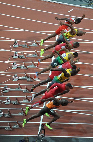
• Gold medal times for Olympic 100 m runners since 1896. Image from Wikimedia Commons http://bit.ly/191adDC

Olympic 100m Data

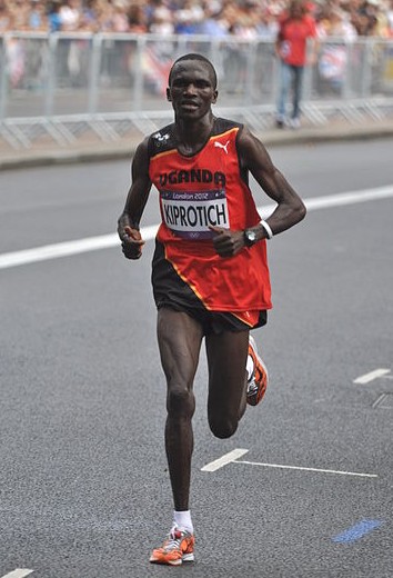
Olympic Marathon Data

Gold medal times for Olympic Marathon since 1896. Marathons before 1924 didn’t have a standardised distance. Present results using pace per km. In 1904 Marathon was badly organised leading to very slow times.

Image from Wikimedia Commons http://bit.ly/16kMKHQ

Olympic Marathon Data

What is Machine Learning?

What is Machine Learning?

What is Machine Learning?

\[\text{data} + \text{model} \xrightarrow{\text{compute}} \text{prediction}\]

• To combine data with a model need:
• a prediction function \(\mappingFunction (\cdot)\) includes our beliefs about the regularities of the universe
• an objective function \(\errorFunction (\cdot)\) defines the cost of misprediction.

Sum of Squares Error

Regression: Linear Releationship

\[\dataScalar_i = m \inputScalar_i + c\]

• \(\dataScalar_i\) : winning pace.

• \(\inputScalar_i\) : year of Olympics.

• \(m\) : rate of improvement over time.

• \(c\) : winning time at year 0.

Overdetermined System

❮ ❯

\(\dataScalar = m\inputScalar + c\)

\(\dataScalar = m\inputScalar + c + \noiseScalar\)

A Probabilistic Process

The Gaussian Density

• Perhaps the most common probability density.

Gaussian Density

Gaussian Density

\[ \gaussianDist{\dataScalar}{\meanScalar}{\dataStd^2} = \frac{1}{\sqrt{2\pi\dataStd^2}} \exp\left(-\frac{(\dataScalar-\meanScalar)^2}{2\dataStd^2}\right) \]

Two Important Gaussian Properties

Sum of Gaussians

Scaling a Gaussian

Laplace’s Idea

A Probabilistic Process

Set the mean of Gaussian to be a function.

Height as a Function of Weight

In the standard Gaussian, parametized by mean and variance.

Make the mean a linear function of an input.

This leads to a regression model. \[ \begin{align*} \dataScalar_i=&\mappingFunction\left(\inputScalar_i\right)+\noiseScalar_i,\\ \noiseScalar_i \sim & \gaussianSamp{0}{\dataStd^2}. \end{align*} \]

Assume \(\dataScalar_i\) is height and \(\inputScalar_i\) is weight.

Data Point Likelihood

Likelihood of an individual data point \[ p\left(\dataScalar_i|\inputScalar_i,m,c\right)=\frac{1}{\sqrt{2\pi \dataStd^2}}\exp\left(-\frac{\left(\dataScalar_i-m\inputScalar_i-c\right)^{2}}{2\dataStd^2}\right). \] Parameters are gradient, \(m\), offset, \(c\) of the function and noise variance \(\dataStd^2\).

Data Set Likelihood

If the noise, \(\epsilon_i\) is sampled independently for each data point. Each data point is independent (given \(m\) and \(c\)). For independent variables: \[ p(\dataVector) = \prod_{i=1}^\numData p(\dataScalar_i) \] \[ p(\dataVector|\inputVector, m, c) = \prod_{i=1}^\numData p(\dataScalar_i|\inputScalar_i, m, c) \]

For Gaussian

i.i.d. assumption \[ p(\dataVector|\inputVector, m, c) = \prod_{i=1}^\numData \frac{1}{\sqrt{2\pi \dataStd^2}}\exp \left(-\frac{\left(\dataScalar_i- m\inputScalar_i-c\right)^{2}}{2\dataStd^2}\right). \] \[ p(\dataVector|\inputVector, m, c) = \frac{1}{\left(2\pi \dataStd^2\right)^{\frac{\numData}{2}}}\exp\left(-\frac{\sum_{i=1}^\numData\left(\dataScalar_i-m\inputScalar_i-c\right)^{2}}{2\dataStd^2}\right). \]

Log Likelihood Function

• Normally work with the log likelihood: \[ L(m,c,\dataStd^{2})=-\frac{\numData}{2}\log 2\pi -\frac{\numData}{2}\log \dataStd^2 -\sum_{i=1}^{\numData}\frac{\left(\dataScalar_i-m\inputScalar_i-c\right)^{2}}{2\dataStd^2}. \]

Consistency of Maximum Likelihood

• If data was really generated according to probability we specified.
• Correct parameters will be recovered in limit as \(\numData \rightarrow \infty\).
• This can be proven through sample based approximations (law of large numbers) of “KL divergences”.
• Mainstay of classical statistics (Wasserman, 2003).

Probabilistic Interpretation of the Error Function

• Probabilistic Interpretation for Error Function is Negative Log Likelihood.
• Minimizing error function is equivalent to maximizing log likelihood.
• Maximizing log likelihood is equivalent to maximizing the likelihood because \(\log\) is monotonic.
• Probabilistic interpretation: Minimizing error function is equivalent to maximum likelihood with respect to parameters.

Error Function

• Negative log likelihood is the error function leading to an error function \[\errorFunction(m,c,\dataStd^{2})=\frac{\numData}{2}\log \dataStd^2+\frac{1}{2\dataStd^2}\sum _{i=1}^{\numData}\left(\dataScalar_i-m\inputScalar_i-c\right)^{2}.\]
• Learning proceeds by minimizing this error function for the data set provided.

Connection: Sum of Squares Error

• Ignoring terms which don’t depend on \(m\) and \(c\) gives \[\errorFunction(m, c) \propto \sum_{i=1}^\numData (\dataScalar_i - \mappingFunction(\inputScalar_i))^2\] where \(\mappingFunction(\inputScalar_i) = m\inputScalar_i + c\).
• This is known as the sum of squares error function.
• Commonly used and is closely associated with the Gaussian likelihood.

Reminder

• Two functions involved:
  • Prediction function: \(\mappingFunction(\inputScalar_i)\)
  • Error, or Objective function: \(\errorFunction(m, c)\)
• Error function depends on parameters through prediction function.

Mathematical Interpretation

• What is the mathematical interpretation?
• There is a cost function.
  • It expresses mismatch between your prediction and reality. \[ \errorFunction(m, c)=\sum_{i=1}^\numData \left(\dataScalar_i - m\inputScalar_i-c\right)^2 \]
  • This is known as the sum of squares error.

Sum of Squares Error

Linear Algebra

Coordinate Descent

Learning is Optimization

• Learning is minimization of the cost function.
• At the minima the gradient is zero.
• Coordinate ascent, find gradient in each coordinate and set to zero. \[\frac{\text{d}\errorFunction(c)}{\text{d}c} = -2\sum_{i=1}^\numData \left(\dataScalar_i- m \inputScalar_i - c \right)\] \[0 = -2\sum_{i=1}^\numData\left(\dataScalar_i- m\inputScalar_i - c \right)\]

Learning is Optimization

• Fixed point equations \[0 = -2\sum_{i=1}^\numData \dataScalar_i +2\sum_{i=1}^\numData m \inputScalar_i +2n c\] \[c = \frac{\sum_{i=1}^\numData \left(\dataScalar_i - m\inputScalar_i\right)}{\numData}\]

Learning is Optimization

• Learning is minimization of the cost function.
• At the minima the gradient is zero.
• Coordinate ascent, find gradient in each coordinate and set to zero. \[\frac{\text{d}\errorFunction(m)}{\text{d}m} = -2\sum_{i=1}^\numData \inputScalar_i\left(\dataScalar_i- m \inputScalar_i - c \right)\] \[0 = -2\sum_{i=1}^\numData \inputScalar_i \left(\dataScalar_i-m \inputScalar_i - c \right)\]

Learning is Optimization

• Fixed point equations \[0 = -2\sum_{i=1}^\numData \inputScalar_i\dataScalar_i+2\sum_{i=1}^\numData m \inputScalar_i^2+2\sum_{i=1}^\numData c\inputScalar_i\] \[m = \frac{\sum_{i=1}^\numData \left(\dataScalar_i -c\right)\inputScalar_i}{\sum_{i=1}^\numData\inputScalar_i^2}\]

\[m^* = \frac{\sum_{i=1}^\numData (\dataScalar_i - c)\inputScalar_i}{\sum_{i=1}^\numData \inputScalar_i^2}\]

Fixed Point Updates

Worked example. \[ \begin{aligned} c^{*}=&\frac{\sum _{i=1}^{\numData}\left(\dataScalar_i-m^{*}\inputScalar_i\right)}{\numData},\\ m^{*}=&\frac{\sum _{i=1}^{\numData}\inputScalar_i\left(\dataScalar_i-c^{*}\right)}{\sum _{i=1}^{\numData}\inputScalar_i^{2}},\\ \left.\dataStd^2\right.^{*}=&\frac{\sum _{i=1}^{\numData}\left(\dataScalar_i-m^{*}\inputScalar_i-c^{*}\right)^{2}}{\numData} \end{aligned} \]

Important Concepts Not Covered

• Other optimization methods:
  • Second order methods, conjugate gradient, quasi-Newton and Newton.
• Effective heuristics such as momentum.
• Local vs global solutions.

Multi-dimensional Inputs

• Multivariate functions involve more than one input.
• Height might be a function of weight and gender.
• There could be other contributory factors.
• Place these factors in a feature vector \(\inputVector_i\).
• Linear function is now defined as \[\mappingFunction(\inputVector_i) = \sum_{j=1}^p w_j \inputScalar_{i, j} + c\]

Vector Notation

• Write in vector notation, \[\mappingFunction(\inputVector_i) = \mappingVector^\top \inputVector_i + c\]
• Can absorb \(c\) into \(\mappingVector\) by assuming extra input \(\inputScalar_0\) which is always 1. \[\mappingFunction(\inputVector_i) = \mappingVector^\top \inputVector_i\]

Objective Functions and Regression

• Classification: map feature to class label.

• Regression: map feature to real value our prediction function is

  \[\mappingFunction(\inputScalar_i) = m\inputScalar_i + c\]

• Need an algorithm to fit it.

• Least squares: minimize an error.

\[\errorFunction(m, c) = \sum_{i=1}^\numData (\dataScalar_i * \mappingFunction(\inputScalar_i))^2\]

Regression

• Create an artifical data set.

We now need to decide on a true value for \(m\) and a true value for \(c\) to use for generating the data.

We can use these values to create our artificial data. The formula \[\dataScalar_i = m\inputScalar_i + c\] is translated to code as follows:

Plot of Data

We can now plot the artifical data we’ve created.

These points lie exactly on a straight line, that’s not very realistic, let’s corrupt them with a bit of Gaussian ‘noise’.

Noise Corrupted Plot

Contour Plot of Error Function

• Visualise the error function surface, create vectors of values.

• create a grid of values to evaluate the error function in 2D.

• compute the error function at each combination of \(c\) and \(m\).

Contour Plot of Error

• We can now make a contour plot.

Steepest Descent

• Minimize the sum of squares error function.
• One way of doing that is gradient descent.
• Initialize with a guess for \(m\) and \(c\)
• update that guess by subtracting a portion of the gradient from the guess.
• Like walking down a hill in the steepest direction of the hill to get to the bottom.

Algorithm

• We start with a guess for \(m\) and \(c\).

Offset Gradient

• Now we need to compute the gradient of the error function, firstly with respect to \(c\),

  \[\frac{\text{d}\errorFunction(m, c)}{\text{d} c} = -2\sum_{i=1}^\numData (\dataScalar_i - m\inputScalar_i - c)\]

• This is computed in python as follows

Deriving the Gradient

To see how the gradient was derived, first note that the \(c\) appears in every term in the sum. So we are just differentiating \((\dataScalar_i - m\inputScalar_i - c)^2\) for each term in the sum. The gradient of this term with respect to \(c\) is simply the gradient of the outer quadratic, multiplied by the gradient with respect to \(c\) of the part inside the quadratic. The gradient of a quadratic is two times the argument of the quadratic, and the gradient of the inside linear term is just minus one. This is true for all terms in the sum, so we are left with the sum in the gradient.

Slope Gradient

The gradient with respect tom \(m\) is similar, but now the gradient of the quadratic’s argument is \(-\inputScalar_i\) so the gradient with respect to \(m\) is

\[\frac{\text{d}\errorFunction(m, c)}{\text{d} m} = -2\sum_{i=1}^\numData \inputScalar_i(\dataScalar_i - m\inputScalar_i - c)\]

which can be implemented in python (numpy) as

Update Equations

• Now we have gradients with respect to \(m\) and \(c\).
• Can update our inital guesses for \(m\) and \(c\) using the gradient.
• We don’t want to just subtract the gradient from \(m\) and \(c\),
• We need to take a small step in the gradient direction.
• Otherwise we might overshoot the minimum.
• We want to follow the gradient to get to the minimum, the gradient changes all the time.

Move in Direction of Gradient

Update Equations

• The step size has already been introduced, it’s again known as the learning rate and is denoted by \(\learnRate\). \[ c_\text{new}\leftarrow c_{\text{old}} - \learnRate \frac{\text{d}\errorFunction(m, c)}{\text{d}c} \]

• gives us an update for our estimate of \(c\) (which in the code we’ve been calling c_star to represent a common way of writing a parameter estimate, \(c^*\)) and \[ m_\text{new} \leftarrow m_{\text{old}} - \learnRate \frac{\text{d}\errorFunction(m, c)}{\text{d}m} \]

• Giving us an update for \(m\).

Update Code

• These updates can be coded as

Iterating Updates

• Fit model by descending gradient.

Gradient Descent Algorithm

❮ ❯

Stochastic Gradient Descent

• If \(\numData\) is small, gradient descent is fine.
• But sometimes (e.g. on the internet \(\numData\) could be a billion.
• Stochastic gradient descent is more similar to perceptron.
• Look at gradient of one data point at a time rather than summing across all data points)
• This gives a stochastic estimate of gradient.

Stochastic Gradient Descent

• The real gradient with respect to \(m\) is given by

  \[\frac{\text{d}\errorFunction(m, c)}{\text{d} m} = -2\sum_{i=1}^\numData \inputScalar_i(\dataScalar_i - m\inputScalar_i - c)\]

  but it has \(\numData\) terms in the sum. Substituting in the gradient we can see that the full update is of the form

  \[m_\text{new} \leftarrow m_\text{old} + 2\learnRate \left[\inputScalar_1 (\dataScalar_1 - m_\text{old}\inputScalar_1 - c_\text{old}) + (\inputScalar_2 (\dataScalar_2 - m_\text{old}\inputScalar_2 - c_\text{old}) + \dots + (\inputScalar_n (\dataScalar_n - m_\text{old}\inputScalar_n - c_\text{old})\right]\]

  This could be split up into lots of individual updates \[m_1 \leftarrow m_\text{old} + 2\learnRate \left[\inputScalar_1 (\dataScalar_1 - m_\text{old}\inputScalar_1 - c_\text{old})\right]\] \[m_2 \leftarrow m_1 + 2\learnRate \left[\inputScalar_2 (\dataScalar_2 - m_\text{old}\inputScalar_2 - c_\text{old})\right]\] \[m_3 \leftarrow m_2 + 2\learnRate \left[\dots\right]\] \[m_n \leftarrow m_{n-1} + 2\learnRate \left[\inputScalar_n (\dataScalar_n - m_\text{old}\inputScalar_n - c_\text{old})\right]\]

which would lead to the same final update.

Updating \(c\) and \(m\)

• In the sum we don’t \(m\) and \(c\) we use for computing the gradient term at each update.
• In stochastic gradient descent we do change them.
• This means it’s not quite the same as steepest desceint.
• But we can present each data point in a random order, like we did for the perceptron.
• This makes the algorithm suitable for large scale web use (recently this domain is know as ‘Big Data’) and algorithms like this are widely used by Google, Microsoft, Amazon, Twitter and Facebook.

Stochastic Gradient Descent

• Or more accurate, since the data is normally presented in a random order we just can write \[ m_\text{new} = m_\text{old} + 2\learnRate\left[\inputScalar_i (\dataScalar_i - m_\text{old}\inputScalar_i - c_\text{old})\right] \]

SGD for Linear Regression

Putting it all together in an algorithm, we can do stochastic gradient descent for our regression data.

❮ ❯

Reflection on Linear Regression and Supervised Learning

Think about:

1. What effect does the learning rate have in the optimization? What’s the effect of making it too small, what’s the effect of making it too big? Do you get the same result for both stochastic and steepest gradient descent?

2. The stochastic gradient descent doesn’t help very much for such a small data set. It’s real advantage comes when there are many, you’ll see this in the lab.

Log Likelihood for Multivariate Regression

The likelihood of a single data point is

Error Function

And a corresponding error function of \[\errorFunction(\mappingVector,\dataStd^2)=\frac{\numData}{2}\log\dataStd^2 + \frac{\sum_{i=1}^{\numData}\left(\dataScalar_i-\mappingVector^{\top}\inputVector_i\right)^{2}}{2\dataStd^2}.\]

Expand the Brackets

\[ \begin{align*} \errorFunction(\mappingVector,\dataStd^2) = & \frac{\numData}{2}\log \dataStd^2 + \frac{1}{2\dataStd^2}\sum _{i=1}^{\numData}\dataScalar_i^{2}-\frac{1}{\dataStd^2}\sum _{i=1}^{\numData}\dataScalar_i\mappingVector^{\top}\inputVector_i\\&+\frac{1}{2\dataStd^2}\sum _{i=1}^{\numData}\mappingVector^{\top}\inputVector_i\inputVector_i^{\top}\mappingVector +\text{const}.\\ = & \frac{\numData}{2}\log \dataStd^2 + \frac{1}{2\dataStd^2}\sum _{i=1}^{\numData}\dataScalar_i^{2}-\frac{1}{\dataStd^2} \mappingVector^\top\sum_{i=1}^{\numData}\inputVector_i\dataScalar_i\\&+\frac{1}{2\dataStd^2} \mappingVector^{\top}\left[\sum _{i=1}^{\numData}\inputVector_i\inputVector_i^{\top}\right]\mappingVector +\text{const}. \end{align*} \]

Multiple Input Solution with Linear Algebra

Design Matrix

Objective Optimisation

Multivariate Derivatives

• We will need some multivariate calculus.
• For now some simple multivariate differentiation: \[\frac{\text{d}{\mathbf{a}^{\top}}{\mappingVector}}{\text{d}\mappingVector}=\mathbf{a}\] and \[\frac{\mappingVector^{\top}\mathbf{A}\mappingVector}{\text{d}\mappingVector}=\left(\mathbf{A}+\mathbf{A}^{\top}\right)\mappingVector\] or if \(\mathbf{A}\) is symmetric (i.e. \(\mathbf{A}=\mathbf{A}^{\top}\)) \[\frac{\text{d}\mappingVector^{\top}\mathbf{A}\mappingVector}{\text{d}\mappingVector}=2\mathbf{A}\mappingVector.\]

Differentiate the Objective

Differentiating with respect to the vector \(\mappingVector\) we obtain \[ \frac{\partial L\left(\mappingVector,\dataStd^2 \right)}{\partial \mappingVector}=\frac{1}{\dataStd^2} \sum _{i=1}^{\numData}\inputVector_i \dataScalar_i-\frac{1}{\dataStd^2} \left[\sum _{i=1}^{\numData}\inputVector_i\inputVector_i^{\top}\right]\mappingVector \] Leading to \[ \mappingVector^{*}=\left[\sum _{i=1}^{\numData}\inputVector_i\inputVector_i^{\top}\right]^{-1}\sum _{i=1}^{\numData}\inputVector_i\dataScalar_i, \]

Differentiate the Objective

Rewrite in matrix notation: \[ \sum_{i=1}^{\numData}\inputVector_i\inputVector_i^\top = \inputMatrix^\top \inputMatrix \] \[ \sum_{i=1}^{\numData}\inputVector_i\dataScalar_i = \inputMatrix^\top \dataVector \]

Update Equation for Global Optimum

Update Equations

• Update for \(\mappingVector^{*}\). \[\mappingVector^{*} = \left(\inputMatrix^\top \inputMatrix\right)^{-1} \inputMatrix^\top \dataVector\]
• The equation for \(\left.\dataStd^2\right.^{*}\) may also be found \[\left.\dataStd^2\right.^{{*}}=\frac{\sum_{i=1}^{\numData}\left(\dataScalar_i-\left.\mappingVector^{*}\right.^{\top}\inputVector_i\right)^{2}}{\numData}.\]

Solving the Multivariate System

}

Reading

• Section 1.3 of Rogers and Girolami (2011) for Matrix & Vector Review.

References

Bishop, C.M., 2006. Pattern recognition and machine learning. springer.
Rogers, S., Girolami, M., 2011. A first course in machine learning. CRC Press.
Wasserman, L.A., 2003. All of statistics. springer, New York.