\[\newcommand{\tk}[1]{} %\newcommand{\tk}[1]{\textbf{TK}: #1} \newcommand{\Amatrix}{\mathbf{A}} \newcommand{\KL}[2]{\text{KL}\left( #1\,\|\,#2 \right)} \newcommand{\Kaast}{\kernelMatrix_{\mathbf{ \ast}\mathbf{ \ast}}} \newcommand{\Kastu}{\kernelMatrix_{\mathbf{ \ast} \inducingVector}} \newcommand{\Kff}{\kernelMatrix_{\mappingFunctionVector \mappingFunctionVector}} \newcommand{\Kfu}{\kernelMatrix_{\mappingFunctionVector \inducingVector}} \newcommand{\Kuast}{\kernelMatrix_{\inducingVector \bf\ast}} \newcommand{\Kuf}{\kernelMatrix_{\inducingVector \mappingFunctionVector}} \newcommand{\Kuu}{\kernelMatrix_{\inducingVector \inducingVector}} \newcommand{\Kuui}{\Kuu^{-1}} \newcommand{\Qaast}{\mathbf{Q}_{\bf \ast \ast}} \newcommand{\Qastf}{\mathbf{Q}_{\ast \mappingFunction}} \newcommand{\Qfast}{\mathbf{Q}_{\mappingFunctionVector \bf \ast}} \newcommand{\Qff}{\mathbf{Q}_{\mappingFunctionVector \mappingFunctionVector}} \newcommand{\aMatrix}{\mathbf{A}} \newcommand{\aScalar}{a} \newcommand{\aVector}{\mathbf{a}} \newcommand{\acceleration}{a} \newcommand{\bMatrix}{\mathbf{B}} \newcommand{\bScalar}{b} \newcommand{\bVector}{\mathbf{b}} \newcommand{\basisFunc}{\phi} \newcommand{\basisFuncVector}{\boldsymbol{ \basisFunc}} \newcommand{\basisFunction}{\phi} \newcommand{\basisLocation}{\mu} \newcommand{\basisMatrix}{\boldsymbol{ \Phi}} \newcommand{\basisScalar}{\basisFunction} \newcommand{\basisVector}{\boldsymbol{ \basisFunction}} \newcommand{\activationFunction}{\phi} \newcommand{\activationMatrix}{\boldsymbol{ \Phi}} \newcommand{\activationScalar}{\basisFunction} \newcommand{\activationVector}{\boldsymbol{ \basisFunction}} \newcommand{\bigO}{\mathcal{O}} \newcommand{\binomProb}{\pi} \newcommand{\cMatrix}{\mathbf{C}} \newcommand{\cbasisMatrix}{\hat{\boldsymbol{ \Phi}}} \newcommand{\cdataMatrix}{\hat{\dataMatrix}} \newcommand{\cdataScalar}{\hat{\dataScalar}} \newcommand{\cdataVector}{\hat{\dataVector}} \newcommand{\centeredKernelMatrix}{\mathbf{ \MakeUppercase{\centeredKernelScalar}}} \newcommand{\centeredKernelScalar}{b} \newcommand{\centeredKernelVector}{\centeredKernelScalar} \newcommand{\centeringMatrix}{\mathbf{H}} \newcommand{\chiSquaredDist}[2]{\chi_{#1}^{2}\left(#2\right)} \newcommand{\chiSquaredSamp}[1]{\chi_{#1}^{2}} \newcommand{\conditionalCovariance}{\boldsymbol{ \Sigma}} \newcommand{\coregionalizationMatrix}{\mathbf{B}} \newcommand{\coregionalizationScalar}{b} \newcommand{\coregionalizationVector}{\mathbf{ \coregionalizationScalar}} \newcommand{\covDist}[2]{\text{cov}_{#2}\left(#1\right)} \newcommand{\covSamp}[1]{\text{cov}\left(#1\right)} \newcommand{\covarianceScalar}{c} \newcommand{\covarianceVector}{\mathbf{ \covarianceScalar}} \newcommand{\covarianceMatrix}{\mathbf{C}} \newcommand{\covarianceMatrixTwo}{\boldsymbol{ \Sigma}} \newcommand{\croupierScalar}{s} \newcommand{\croupierVector}{\mathbf{ \croupierScalar}} \newcommand{\croupierMatrix}{\mathbf{ \MakeUppercase{\croupierScalar}}} \newcommand{\dataDim}{p} \newcommand{\dataIndex}{i} \newcommand{\dataIndexTwo}{j} \newcommand{\dataMatrix}{\mathbf{Y}} \newcommand{\dataScalar}{y} \newcommand{\dataSet}{\mathcal{D}} \newcommand{\dataStd}{\sigma} \newcommand{\dataVector}{\mathbf{ \dataScalar}} \newcommand{\decayRate}{d} \newcommand{\degreeMatrix}{\mathbf{ \MakeUppercase{\degreeScalar}}} \newcommand{\degreeScalar}{d} \newcommand{\degreeVector}{\mathbf{ \degreeScalar}} % Already defined by latex %\newcommand{\det}[1]{\left|#1\right|} \newcommand{\diag}[1]{\text{diag}\left(#1\right)} \newcommand{\diagonalMatrix}{\mathbf{D}} \newcommand{\diff}[2]{\frac{\text{d}#1}{\text{d}#2}} \newcommand{\diffTwo}[2]{\frac{\text{d}^2#1}{\text{d}#2^2}} \newcommand{\displacement}{x} \newcommand{\displacementVector}{\textbf{\displacement}} \newcommand{\distanceMatrix}{\mathbf{ \MakeUppercase{\distanceScalar}}} \newcommand{\distanceScalar}{d} \newcommand{\distanceVector}{\mathbf{ \distanceScalar}} \newcommand{\eigenvaltwo}{\ell} \newcommand{\eigenvaltwoMatrix}{\mathbf{L}} \newcommand{\eigenvaltwoVector}{\mathbf{l}} \newcommand{\eigenvalue}{\lambda} \newcommand{\eigenvalueMatrix}{\boldsymbol{ \Lambda}} \newcommand{\eigenvalueVector}{\boldsymbol{ \lambda}} \newcommand{\eigenvector}{\mathbf{ \eigenvectorScalar}} \newcommand{\eigenvectorMatrix}{\mathbf{U}} \newcommand{\eigenvectorScalar}{u} \newcommand{\eigenvectwo}{\mathbf{v}} \newcommand{\eigenvectwoMatrix}{\mathbf{V}} \newcommand{\eigenvectwoScalar}{v} \newcommand{\entropy}[1]{\mathcal{H}\left(#1\right)} \newcommand{\errorFunction}{E} \newcommand{\expDist}[2]{\left<#1\right>_{#2}} \newcommand{\expSamp}[1]{\left<#1\right>} \newcommand{\expectation}[1]{\left\langle #1 \right\rangle } \newcommand{\expectationDist}[2]{\left\langle #1 \right\rangle _{#2}} \newcommand{\expectedDistanceMatrix}{\mathcal{D}} \newcommand{\eye}{\mathbf{I}} \newcommand{\fantasyDim}{r} \newcommand{\fantasyMatrix}{\mathbf{ \MakeUppercase{\fantasyScalar}}} \newcommand{\fantasyScalar}{z} \newcommand{\fantasyVector}{\mathbf{ \fantasyScalar}} \newcommand{\featureStd}{\varsigma} \newcommand{\gammaCdf}[3]{\mathcal{GAMMA CDF}\left(#1|#2,#3\right)} \newcommand{\gammaDist}[3]{\mathcal{G}\left(#1|#2,#3\right)} \newcommand{\gammaSamp}[2]{\mathcal{G}\left(#1,#2\right)} \newcommand{\gaussianDist}[3]{\mathcal{N}\left(#1|#2,#3\right)} \newcommand{\gaussianSamp}[2]{\mathcal{N}\left(#1,#2\right)} \newcommand{\given}{|} \newcommand{\half}{\frac{1}{2}} \newcommand{\heaviside}{H} \newcommand{\hiddenMatrix}{\mathbf{ \MakeUppercase{\hiddenScalar}}} \newcommand{\hiddenScalar}{h} \newcommand{\hiddenVector}{\mathbf{ \hiddenScalar}} \newcommand{\identityMatrix}{\eye} \newcommand{\inducingInputScalar}{z} \newcommand{\inducingInputVector}{\mathbf{ \inducingInputScalar}} \newcommand{\inducingInputMatrix}{\mathbf{Z}} \newcommand{\inducingScalar}{u} \newcommand{\inducingVector}{\mathbf{ \inducingScalar}} \newcommand{\inducingMatrix}{\mathbf{U}} \newcommand{\inlineDiff}[2]{\text{d}#1/\text{d}#2} \newcommand{\inputDim}{q} \newcommand{\inputMatrix}{\mathbf{X}} \newcommand{\inputScalar}{x} \newcommand{\inputSpace}{\mathcal{X}} \newcommand{\inputVals}{\inputVector} \newcommand{\inputVector}{\mathbf{ \inputScalar}} \newcommand{\iterNum}{k} \newcommand{\kernel}{\kernelScalar} \newcommand{\kernelMatrix}{\mathbf{K}} \newcommand{\kernelScalar}{k} \newcommand{\kernelVector}{\mathbf{ \kernelScalar}} \newcommand{\kff}{\kernelScalar_{\mappingFunction \mappingFunction}} \newcommand{\kfu}{\kernelVector_{\mappingFunction \inducingScalar}} \newcommand{\kuf}{\kernelVector_{\inducingScalar \mappingFunction}} \newcommand{\kuu}{\kernelVector_{\inducingScalar \inducingScalar}} \newcommand{\lagrangeMultiplier}{\lambda} \newcommand{\lagrangeMultiplierMatrix}{\boldsymbol{ \Lambda}} \newcommand{\lagrangian}{L} \newcommand{\laplacianFactor}{\mathbf{ \MakeUppercase{\laplacianFactorScalar}}} \newcommand{\laplacianFactorScalar}{m} \newcommand{\laplacianFactorVector}{\mathbf{ \laplacianFactorScalar}} \newcommand{\laplacianMatrix}{\mathbf{L}} \newcommand{\laplacianScalar}{\ell} \newcommand{\laplacianVector}{\mathbf{ \ell}} \newcommand{\latentDim}{q} \newcommand{\latentDistanceMatrix}{\boldsymbol{ \Delta}} \newcommand{\latentDistanceScalar}{\delta} \newcommand{\latentDistanceVector}{\boldsymbol{ \delta}} \newcommand{\latentForce}{f} \newcommand{\latentFunction}{u} \newcommand{\latentFunctionVector}{\mathbf{ \latentFunction}} \newcommand{\latentFunctionMatrix}{\mathbf{ \MakeUppercase{\latentFunction}}} \newcommand{\latentIndex}{j} \newcommand{\latentScalar}{z} \newcommand{\latentVector}{\mathbf{ \latentScalar}} \newcommand{\latentMatrix}{\mathbf{Z}} \newcommand{\learnRate}{\eta} \newcommand{\lengthScale}{\ell} \newcommand{\rbfWidth}{\ell} \newcommand{\likelihoodBound}{\mathcal{L}} \newcommand{\likelihoodFunction}{L} \newcommand{\locationScalar}{\mu} \newcommand{\locationVector}{\boldsymbol{ \locationScalar}} \newcommand{\locationMatrix}{\mathbf{M}} \newcommand{\variance}[1]{\text{var}\left( #1 \right)} \newcommand{\mappingFunction}{f} \newcommand{\mappingFunctionMatrix}{\mathbf{F}} \newcommand{\mappingFunctionTwo}{g} \newcommand{\mappingFunctionTwoMatrix}{\mathbf{G}} \newcommand{\mappingFunctionTwoVector}{\mathbf{ \mappingFunctionTwo}} \newcommand{\mappingFunctionVector}{\mathbf{ \mappingFunction}} \newcommand{\scaleScalar}{s} \newcommand{\mappingScalar}{w} \newcommand{\mappingVector}{\mathbf{ \mappingScalar}} \newcommand{\mappingMatrix}{\mathbf{W}} \newcommand{\mappingScalarTwo}{v} \newcommand{\mappingVectorTwo}{\mathbf{ \mappingScalarTwo}} \newcommand{\mappingMatrixTwo}{\mathbf{V}} \newcommand{\maxIters}{K} \newcommand{\meanMatrix}{\mathbf{M}} \newcommand{\meanScalar}{\mu} \newcommand{\meanTwoMatrix}{\mathbf{M}} \newcommand{\meanTwoScalar}{m} \newcommand{\meanTwoVector}{\mathbf{ \meanTwoScalar}} \newcommand{\meanVector}{\boldsymbol{ \meanScalar}} \newcommand{\mrnaConcentration}{m} \newcommand{\naturalFrequency}{\omega} \newcommand{\neighborhood}[1]{\mathcal{N}\left( #1 \right)} \newcommand{\neilurl}{http://inverseprobability.com/} \newcommand{\noiseMatrix}{\boldsymbol{ E}} \newcommand{\noiseScalar}{\epsilon} \newcommand{\noiseVector}{\boldsymbol{ \epsilon}} \newcommand{\norm}[1]{\left\Vert #1 \right\Vert} \newcommand{\normalizedLaplacianMatrix}{\hat{\mathbf{L}}} \newcommand{\normalizedLaplacianScalar}{\hat{\ell}} \newcommand{\normalizedLaplacianVector}{\hat{\mathbf{ \ell}}} \newcommand{\numActive}{m} \newcommand{\numBasisFunc}{m} \newcommand{\numComponents}{m} \newcommand{\numComps}{K} \newcommand{\numData}{n} \newcommand{\numFeatures}{K} \newcommand{\numHidden}{h} \newcommand{\numInducing}{m} \newcommand{\numLayers}{\ell} \newcommand{\numNeighbors}{K} \newcommand{\numSequences}{s} \newcommand{\numSuccess}{s} \newcommand{\numTasks}{m} \newcommand{\numTime}{T} \newcommand{\numTrials}{S} \newcommand{\outputIndex}{j} \newcommand{\paramVector}{\boldsymbol{ \theta}} \newcommand{\parameterMatrix}{\boldsymbol{ \Theta}} \newcommand{\parameterScalar}{\theta} \newcommand{\parameterVector}{\boldsymbol{ \parameterScalar}} \newcommand{\partDiff}[2]{\frac{\partial#1}{\partial#2}} \newcommand{\precisionScalar}{j} \newcommand{\precisionVector}{\mathbf{ \precisionScalar}} \newcommand{\precisionMatrix}{\mathbf{J}} \newcommand{\pseudotargetScalar}{\widetilde{y}} \newcommand{\pseudotargetVector}{\mathbf{ \pseudotargetScalar}} \newcommand{\pseudotargetMatrix}{\mathbf{ \widetilde{Y}}} \newcommand{\rank}[1]{\text{rank}\left(#1\right)} \newcommand{\rayleighDist}[2]{\mathcal{R}\left(#1|#2\right)} \newcommand{\rayleighSamp}[1]{\mathcal{R}\left(#1\right)} \newcommand{\responsibility}{r} \newcommand{\rotationScalar}{r} \newcommand{\rotationVector}{\mathbf{ \rotationScalar}} \newcommand{\rotationMatrix}{\mathbf{R}} \newcommand{\sampleCovScalar}{s} \newcommand{\sampleCovVector}{\mathbf{ \sampleCovScalar}} \newcommand{\sampleCovMatrix}{\mathbf{s}} \newcommand{\scalarProduct}[2]{\left\langle{#1},{#2}\right\rangle} \newcommand{\sign}[1]{\text{sign}\left(#1\right)} \newcommand{\sigmoid}[1]{\sigma\left(#1\right)} \newcommand{\singularvalue}{\ell} \newcommand{\singularvalueMatrix}{\mathbf{L}} \newcommand{\singularvalueVector}{\mathbf{l}} \newcommand{\sorth}{\mathbf{u}} \newcommand{\spar}{\lambda} \newcommand{\trace}[1]{\text{tr}\left(#1\right)} \newcommand{\BasalRate}{B} \newcommand{\DampingCoefficient}{C} \newcommand{\DecayRate}{D} \newcommand{\Displacement}{X} \newcommand{\LatentForce}{F} \newcommand{\Mass}{M} \newcommand{\Sensitivity}{S} \newcommand{\basalRate}{b} \newcommand{\dampingCoefficient}{c} \newcommand{\mass}{m} \newcommand{\sensitivity}{s} \newcommand{\springScalar}{\kappa} \newcommand{\springVector}{\boldsymbol{ \kappa}} \newcommand{\springMatrix}{\boldsymbol{ \mathcal{K}}} \newcommand{\tfConcentration}{p} \newcommand{\tfDecayRate}{\delta} \newcommand{\tfMrnaConcentration}{f} \newcommand{\tfVector}{\mathbf{ \tfConcentration}} \newcommand{\velocity}{v} \newcommand{\sufficientStatsScalar}{g} \newcommand{\sufficientStatsVector}{\mathbf{ \sufficientStatsScalar}} \newcommand{\sufficientStatsMatrix}{\mathbf{G}} \newcommand{\switchScalar}{s} \newcommand{\switchVector}{\mathbf{ \switchScalar}} \newcommand{\switchMatrix}{\mathbf{S}} \newcommand{\tr}[1]{\text{tr}\left(#1\right)} \newcommand{\loneNorm}[1]{\left\Vert #1 \right\Vert_1} \newcommand{\ltwoNorm}[1]{\left\Vert #1 \right\Vert_2} \newcommand{\onenorm}[1]{\left\vert#1\right\vert_1} \newcommand{\twonorm}[1]{\left\Vert #1 \right\Vert} \newcommand{\vScalar}{v} \newcommand{\vVector}{\mathbf{v}} \newcommand{\vMatrix}{\mathbf{V}} \newcommand{\varianceDist}[2]{\text{var}_{#2}\left( #1 \right)} % Already defined by latex %\newcommand{\vec}{#1:} \newcommand{\vecb}[1]{\left(#1\right):} \newcommand{\weightScalar}{w} \newcommand{\weightVector}{\mathbf{ \weightScalar}} \newcommand{\weightMatrix}{\mathbf{W}} \newcommand{\weightedAdjacencyMatrix}{\mathbf{A}} \newcommand{\weightedAdjacencyScalar}{a} \newcommand{\weightedAdjacencyVector}{\mathbf{ \weightedAdjacencyScalar}} \newcommand{\onesVector}{\mathbf{1}} \newcommand{\zerosVector}{\mathbf{0}} \]

Generalization: Model Validation

Neil D. Lawrence

University of Sheffield

Review

  • Last time: introduced basis functions.
  • Showed how to maximize the likelihood of a non-linear model that’s linear in parameters.
  • Explored the different characteristics of different basis function models
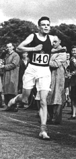
Alan Turing

Probability Winning Olympics?

  • He was a formidable Marathon runner.
  • In 1946 he ran a time 2 hours 46 minutes.
    • That’s a pace of 3.95 min/km.
  • What is the probability he would have won an Olympics if one had been held in 1946?

Expected Loss

\[ R(\mappingVector) = \int L(\dataScalar, \inputScalar, \mappingVector) \mathbb{P}(\dataScalar, \inputScalar) \text{d}\dataScalar \text{d}\inputScalar. \]

Sample Based Approximations

  • Sample based approximation: replace true expectation with sum over samples. \[ \int \mappingFunction(z) p(z) \text{d}z\approx \frac{1}{s}\sum_{i=1}^s \mappingFunction(z_i). \]

  • Allows us to approximate true integral with a sum \[ R(\mappingVector) \approx \frac{1}{\numData}\sum_{i=1}^{\numData} L(\dataScalar_i, \inputScalar_i, \mappingVector). \]

Empirical Risk Minimization

  • If the loss is the squared loss \[ L(\dataScalar, \inputScalar, \mappingVector) = (\dataScalar-\mappingVector^\top\boldsymbol{\phi}(\inputScalar))^2, \]
  • This recovers the empirical risk \[ R(\mappingVector) \approx \frac{1}{\numData} \sum_{i=1}^{\numData} (\dataScalar_i - \mappingVector^\top \boldsymbol{\phi}(\inputScalar_i))^2 \]

Estimating Risk through Validation

Validation

Olympic Marathon Data

  • Gold medal times for Olympic Marathon since 1896.
  • Marathons before 1924 didn’t have a standardised distance.
  • Present results using pace per km.
  • In 1904 Marathon was badly organised leading to very slow times.
Image from Wikimedia Commons http://bit.ly/16kMKHQ

Olympic Marathon Data

Validation on the Olympic Marathon Data

Polynomial Fit: Training Error

The next thing we’ll do is consider a quadratic fit. We will compute the training error for the two fits.

Polynomial Fits to Olympics Data

Hold Out Validation on Olympic Marathon Data

Overfitting

  • Increase number of basis functions we obtain a better ‘fit’ to the data.
  • How will the model perform on previously unseen data?
  • Let’s consider predicting the future.

Future Prediction: Extrapolation

Extrapolation

  • Here we are training beyond where the model has learnt.
  • This is known as extrapolation.
  • Extrapolation is predicting into the future here, but could be:
    • Predicting back to the unseen past (pre 1892)
    • Spatial prediction (e.g. Cholera rates outside Manchester given rates inside Manchester).

Interpolation

  • Predicting the wining time for 1946 Olympics is interpolation.
  • This is because we have times from 1936 and 1948.
  • If we want a model for interpolation how can we test it?
  • One trick is to sample the validation set from throughout the data set.

Future Prediction: Interpolation

Choice of Validation Set

  • The choice of validation set should reflect how you will use the model in practice.
  • For extrapolation into the future we tried validating with data from the future.
  • For interpolation we chose validation set from data.
  • For different validation sets we could get different results.

Leave One Out Validation

Leave One Out Error

  • Take training set and remove one point.
  • Train on the remaining data.
  • Compute the error on the point you removed (which wasn’t in the training data).
  • Do this for each point in the training set in turn.
  • Average the resulting error.
  • This is the leave one out error.

Leave One Out Validation

fold

num basis

num basis

num basis

num basis

num basis

num basis

\(k\)-fold Cross Validation

  • Leave one out error can be very time consuming.
  • Need to train your algorithm \(\numData\) times.
  • An alternative: \(k\) fold cross validation.

\(k\)-fold Cross Validation

fold

num basis

num basis

num basis

num basis

num basis

num basis

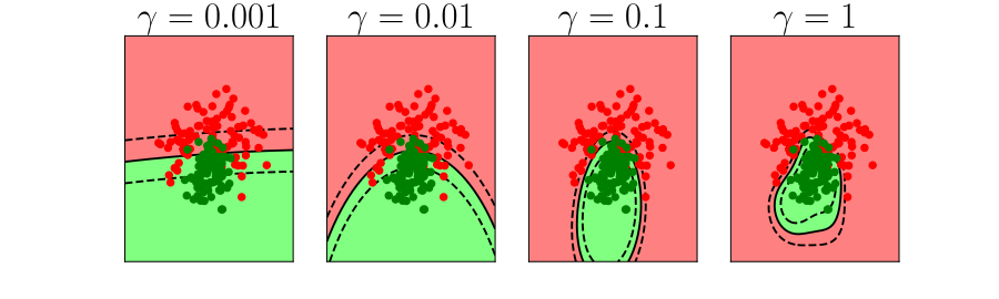
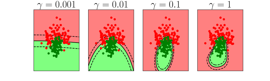
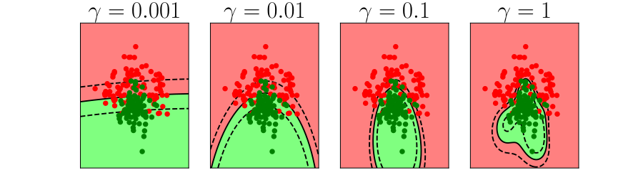
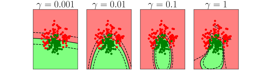
Bias Variance Decomposition

Expected test error for different variations of the training data sampled from, \(\Pr(\dataVector, \dataScalar)\) \[\mathbb{E}\left[ \left(\dataScalar - \mappingFunction^*(\dataVector)\right)^2 \right]\] Decompose as \[\mathbb{E}\left[ \left(\dataScalar - \mappingFunction(\dataVector)\right)^2 \right] = \text{bias}\left[\mappingFunction^*(\dataVector)\right]^2 + \text{variance}\left[\mappingFunction^*(\dataVector)\right] +\sigma^2\]

Bias

  • Given by \[\text{bias}\left[\mappingFunction^*(\dataVector)\right] = \mathbb{E}\left[\mappingFunction^*(\dataVector)\right] * \mappingFunction(\dataVector)\]
  • Error due to bias comes from a model that’s too simple.

Variance

  • Given by \[\text{variance}\left[\mappingFunction^*(\dataVector)\right] = \mathbb{E}\left[\left(\mappingFunction^*(\dataVector) - \mathbb{E}\left[\mappingFunction^*(\dataVector)\right]\right)^2\right]\]
  • Slight variations in the training set cause changes in the prediction. Error due to variance is error in the model due to an overly complex model.

Figure: simple models on left complex models on right

Further Reading

  • Section 1.5 of Rogers and Girolami (2011)

Thanks!

References

Rogers, S., Girolami, M., 2011. A first course in machine learning. CRC Press.