What is Machine Learning?
data : observations, could be actively or passively acquired (meta-data).
model : assumptions, based on previous experience (other data! transfer learning etc), or beliefs about the regularities of the universe. Inductive bias.
prediction : an action to be taken or a categorization or a quality score.
Fitting Data
- data
import numpy as np

# Create some data
x = np.array([1, 3])
y = np.array([3, 1])
- model $$y=mx + c$$
Model Fitting
$$m = \frac{y_2- y_1}{x_2-x_1}$$$$ c = y_1 - m x_1 $$xvals = np.linspace(0, 5, 2);
m = (y[1]-y[0])/(x[1]-x[0]);
c = y[0]-m*x[0];
yvals = m*xvals+c;
%matplotlib inline
import matplotlib.pyplot as plt
xvals = np.linspace(0, 5, 2);

m = (y[1]-y[0])/(x[1]-x[0]);
c = y[0]-m*x[0];

yvals = m*xvals+c;
ylim = np.array([0, 5])
xlim = np.array([0, 5])
f, ax = plt.subplots(1,1,figsize=(5,5))
a = ax.plot(xvals, yvals, '-', linewidth=3);
ax.set_xlim(xlim)
ax.set_ylim(ylim)
plt.xlabel('$x$', fontsize=30)
plt.ylabel('$y$',fontsize=30)
plt.text(4, 4, '$y=mx+c$', horizontalalignment='center', verticalalignment='bottom', fontsize=30)
plt.savefig('diagrams/straight_line1.svg')
ctext = ax.text(0.15, c+0.15, '$c$', horizontalalignment='center', verticalalignment='bottom', fontsize=20)
xl = np.array([1.5, 2.5])
yl = xl*m + c;
mhand = ax.plot([xl[0], xl[1]], [yl.min(), yl.min()], color=[0, 0, 0])
mhand2 = ax.plot([xl.min(), xl.min()], [yl[0], yl[1]], color=[0, 0, 0])
mtext = ax.text(xl.mean(), yl.min()-0.2, '$m$', horizontalalignment='center', verticalalignment='bottom',fontsize=20);
plt.savefig('diagrams/straight_line2.svg')
a2 = ax.plot(x, y, '.', markersize=20, linewidth=3, color=[1, 0, 0])
plt.savefig('diagrams/straight_line3.svg')
xs = 2
ys = m*xs + c + 0.3
ast = ax.plot(xs, ys, '.', markersize=20, linewidth=3, color=[0, 1, 0])
plt.savefig('diagrams/straight_line4.svg')
m = (y[1]-ys)/(x[1]-xs);
c = ys-m*xs;
yvals = m*xvals+c;
for i in a:
i.set_visible(False)
for i in mhand:
i.set_visible(False)
for i in mhand2:
i.set_visible(False)
mtext.set_visible(False)
ctext.set_visible(False)
a3 = ax.plot(xvals, yvals, '-', linewidth=2, color=[0, 0, 1])
for i in ast:
i.set_color([1, 0, 0])
plt.savefig('diagrams/straight_line5.svg')
m = (ys-y[0])/(xs-x[0])
c = y[0]-m*x[0]
yvals = m*xvals+c
for i in a3:
i.set_visible(False)
a4 = ax.plot(xvals, yvals, '-', linewidth=2, color=[0, 0, 1]);
for i in ast:
i.set_color([1, 0, 0])
plt.savefig('diagrams/straight_line6.svg')
for i in a:
i.set_visible(True)
for i in a3:
i.set_visible(True)
plt.savefig('diagrams/straight_line7.svg')
import pods
pods.notebook.display_plots('straight_line{plot}.svg',
                            directory='./diagrams', plot=(1, 7))
$y = mx + c$
point 1: $x = 1$, $y=3$ $$3 = m + c$$ point 2: $x = 3$, $y=1$ $$1 = 3m + c$$ point 3: $x = 2$, $y=2.5$ $$2.5 = 2m + c$$


$y = mx + c + \epsilon$
point 1: $x = 1$, $y=3$ $$3 = m + c + \epsilon_1$$
point 2: $x = 3$, $y=1$ $$1 = 3m + c + \epsilon_2$$
point 3: $x = 2$, $y=2.5$ $$2.5 = 2m + c + \epsilon_3$$
Regression Examples
Predict a real value, $y_i$ given some inputs $x_i$.
Predict quality of meat given spectral measurements (Tecator data).
Radiocarbon dating, the C14 calibration curve: predict age given quantity of C14 isotope.
Predict quality of different Go or Backgammon moves given expert rated training data.
Olympic 100m Data
- Gold medal times for Olympic 100 m runners since 1896.
 Image from Wikimedia Commons http://bit.ly/191adDC
Olympic 100m Data
data = pods.datasets.olympic_100m_men()
f, ax = plt.subplots(figsize=(7,7))
ax.plot(data['X'], data['Y'], 'ro', markersize=10)
[<matplotlib.lines.Line2D at 0x109316208>]
Olympic Marathon Data
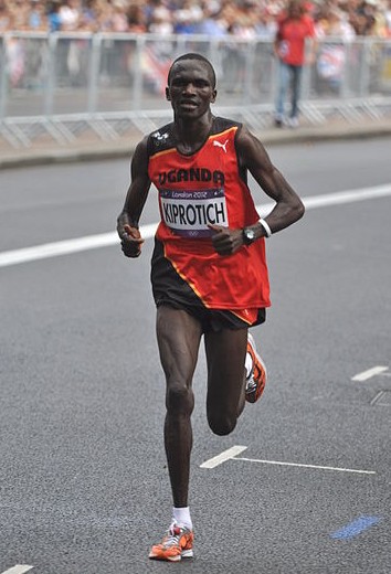 Image from Wikimedia Commons http://bit.ly/16kMKHQ
Olympic Marathon Data
Gold medal times for Olympic Marathon since 1896.
Marathons before 1924 didn’t have a standardised distance.
Present results using pace per km.
In 1904 Marathon was badly organised leading to very slow times.
Olympic Marathon Data
data = pods.datasets.olympic_marathon_men()
f, ax = plt.subplots(figsize=(7,7))
ax.plot(data['X'], data['Y'], 'ro',markersize=10)
[<matplotlib.lines.Line2D at 0x114702ef0>]
What is Machine Learning?
$$ \text{data} + \text{model} = \text{prediction}$$$\text{data}$ : observations, could be actively or passively acquired (meta-data).
$\text{model}$ : assumptions, based on previous experience (other data! transfer learning etc), or beliefs about the regularities of the universe. Inductive bias.
$\text{prediction}$ : an action to be taken or a categorization or a quality score.
Regression: Linear Releationship
$$y_i = m x_i + c$$$y_i$ : winning time/pace.
$x_i$ : year of Olympics.
$m$ : rate of improvement over time.
$c$ : winning time at year 0.
Overdetermined System
$y = mx + c$
point 1: $x = 1$, $y=3$ $$3 = m + c$$ point 2: $x = 3$, $y=1$ $$1 = 3m + c$$ point 3: $x = 2$, $y=2.5$ $$2.5 = 2m + c$$

$y = mx + c + \epsilon$
point 1: $x = 1$, $y=3$ $$3 = m + c + \epsilon_1$$
point 2: $x = 3$, $y=1$ $$1 = 3m + c + \epsilon_2$$
point 3: $x = 2$, $y=2.5$ $$2.5 = 2m + c + \epsilon_3$$
The Gaussian Density
- Perhaps the most common probability density. \begin{align} p(y| \mu, \sigma^2) & = \frac{1}{\sqrt{2\pi\sigma^2}}\exp\left(-\frac{(y - \mu)^2}{2\sigma^2}\right)\ & \buildrel\triangle\over = \mathcal{N}(y|\mu, \sigma^2) \end{align}
- The Gaussian density.
Gaussian Density
The Gaussian PDF with $\mu=1.7$ and variance $\sigma^2=
0.0225$. Mean shown as red line. It could represent the heights of a population of
students.
Gaussian Density
$$ \mathcal{N}(y|\mu, \sigma^2) = \frac{1}{\sqrt{2\pi\sigma^2}} \exp\left(-\frac{(y-\mu)^2}{2\sigma^2}\right) $$$\sigma^2$ is the variance of the density and $\mu$ is the mean.
Height as a Function of Weight
In the standard Gaussian, parametized by mean and variance.
Make the mean a linear function of an input.
This leads to a regression model. \begin{align*} y_i=&f\left(x_i\right)+\epsilon_i,\
\epsilon_i \sim &\mathcal{N}(0, \sigma^2).\end{align*}
Assume $y_i$ is height and $x_i$ is weight.
Data Point Likelihood
Likelihood of an individual data point $$p\left(y_i|x_i,m,c\right)=\frac{1}{\sqrt{2\pi \sigma^2}}\exp \left(-\frac{\left(y_i-mx_i-c\right)^{2}}{2\sigma^2}\right).$$
Parameters are gradient, $m$, offset, $c$ of the function and noise variance $\sigma^2$.
Data Set Likelihood
If the noise, $\epsilon_i$ is sampled independently for each data point.
Each data point is independent (given $m$ and $c$).
For independent variables: $$p(\mathbf{y}) = \prod_{i=1}^n p(y_i)$$ $$p(\mathbf{y}|\mathbf{x}, m, c) = \prod_{i=1}^n p(y_i|x_i, m, c)$$
For Gaussian
i.i.d. assumption
$$p(\mathbf{y}|\mathbf{x}, m, c) = \prod_{i=1}^n \frac{1}{\sqrt{2\pi \sigma^2}}\exp \left(-\frac{\left(y_i-mx_i-c\right)^{2}}{2\sigma^2}\right).$$ $$p(\mathbf{y}|\mathbf{x}, m, c) = \frac{1}{\left(2\pi \sigma^2\right)^{\frac{n}{2}}}\exp \left(-\frac{\sum_{i=1}^n\left(y_i-mx_i-c\right)^{2}}{2\sigma^2}\right).$$
Log Likelihood Function
- Normally work with the log likelihood: $$L(m,c,\sigma^{2})=-\frac{n}{2}\log 2\pi -\frac{n}{2}\log \sigma^2 -\sum _{i=1}^{n}\frac{\left(y_i-mx_i-c\right)^{2}}{2\sigma^2}.$$
Error Function
Negative log likelihood is the error function leading to an error function $$E(m,c,\sigma^{2})=\frac{n}{2}\log \sigma^2 +\frac{1}{2\sigma^2}\sum _{i=1}^{n}\left(y_i-mx_i-c\right)^{2}.$$
Learning proceeds by minimizing this error function for the data set provided.
Connection: Sum of Squares Error
Ignoring terms which don’t depend on $m$ and $c$ gives $$E(m, c) \propto \sum_{i=1}^n (y_i - f(x_i))^2$$ where $f(x_i) = mx_i + c$.
This is known as the sum of squares error function.
Commonly used and is closely associated with the Gaussian likelihood.
Reminder
- Two functions involved:
- Prediction function: $f(x_i)$
- Error, or Objective function: $E(m, c)$
- Error function depends on parameters through prediction function.
Mathematical Interpretation
What is the mathematical interpretation?
There is a cost function.
It expresses mismatch between your prediction and reality. $$E(m, c)=\sum_{i=1}^n \left(y_i - mx_i -c\right)^2$$
This is known as the sum of squares error.
Nonlinear Regression
Problem with Linear Regression—$\mathbf{x}$ may not be linearly related to $\mathbf{y}$.
Potential solution: create a feature space: define $\phi(\mathbf{x})$ where $\phi(\cdot)$ is a nonlinear function of $\mathbf{x}$.
Model for target is a linear combination of these nonlinear functions $$f(\mathbf{x}) = \sum_{j=1}^k w_j \phi_j(\mathbf{x})$$
Quadratic Basis
- Basis functions can be global. E.g. quadratic basis: $$\boldsymbol{\phi} = [1, x, x^2]$$
pods.notebook.display_plots('polynomial_basis{num_basis}.svg', directory='./diagrams', num_basis=(1,3))
Functions Derived from Quadratic Basis
$$f(x) = {\color{\redColor}w_0} + {\color{\magentaColor}w_1x} + {\color{\blueColor}w_2 x^2}$$pods.notebook.display_plots('polynomial_function{func_num}.svg', directory='./diagrams', func_num=(1,3))
Radial Basis Functions
- Or they can be local. E.g. radial (or Gaussian) basis $$\phi_j(x) = \exp\left(-\frac{(x-\mu_j)^2}{\ell^2}\right)$$
pods.notebook.display_plots('radial_basis{num_basis}.svg', directory='./diagrams', num_basis=(1,3))
Functions Derived from Radial Basis
$$f(x) = {\color{\redColor}w_1 e^{-2(x+1)^2}} + {\color{\magentaColor}w_2e^{-2x^2}} + {\color{\blueColor}w_3 e^{-2(x-1)^2}}$$pods.notebook.display_plots('radial_function{func_num}.svg', directory='./diagrams', func_num=(1,3))
Basis Function Models
- The prediction function is now defined as $$f(\mathbf{x}_i) = \sum_{j=1}^m w_j \phi_{i, j}$$
Vector Notation
- Write in vector notation, $$f(\mathbf{x}_i) = \mathbf{w}^\top \boldsymbol{\phi}_i$$
Log Likelihood for Basis Function Model
- The likelihood of a single data point is
$$p\left(y_i|x_i\right)=\frac{1}{\sqrt{2\pi\sigma^2}}\exp
\left(-\frac{\left(y_i-\mathbf{w}^{\top}\boldsymbol{\phi}_i\right)^{2}}{2\sigma^2}\right).$$
Log Likelihood for Basis Function Model
- Leading to a log likelihood for the data set of
$$L(\mathbf{w},\sigma^2)= -\frac{n}{2}\log \sigma^2
  -\frac{n}{2}\log 2\pi -\frac{\sum
    _{i=1}^{n}\left(y_i-\mathbf{w}^{\top}\boldsymbol{\phi}_i\right)^{2}}{2\sigma^2}.$$
Objective Function
- And a corresponding objective function of the form
$$E(\mathbf{w},\sigma^2)= \frac{n}{2}\log
    \sigma^2 + \frac{\sum
      _{i=1}^{n}\left(y_i-\mathbf{w}^{\top}\boldsymbol{\phi}_i\right)^{2}}{2\sigma^2}.$$
Polynomial Fits to Olympic Data
pods.notebook.display_plots('olympic_LM_polynomial{num_basis}.svg', directory='./diagrams', num_basis=(1,7))
Polynomial Fits to Olymics Data
pods.notebook.display_plots('olympic_LM_polynomial{num_basis}.svg',
                            directory='./diagrams', num_basis=(1, max_basis))
Overfitting
- Increase number of basis functions we obtain a better 'fit' to the data.
- How will the model perform on previously unseen data?
- Let's consider predicting the future.
pods.notebook.display_plots('olympic_val_LM_polynomial{num_basis}.svg',
                            directory='./diagrams', num_basis=(1, max_basis))
Extrapolation
- Here we are training beyond where the model has learnt.
- This is known as extrapolation.
- Extrapolation is predicting into the future here, but could be:
- Predicting back to the unseen past (pre 1892)
- Spatial prediction (e.g. Cholera rates outside Manchester given rates inside Manchester).
Alan Turing
- He was a formidable Marathon runner.
- In 1946 he ran a time 2 hours 46 minutes.
- What is the probability he would have won an Olympics if one had been held in 1946?

*Alan Turing, in 1946 he was only 11 minutes slower than the winner of the 1948 games. Would he have won a hypothetical games held in 1946? Source: [Alan Turing Internet Scrapbook](http://www.turing.org.uk/scrapbook/run.html).*
Interpolation
- Predicting the wining time for 1946 Olympics is interpolation.
- This is because we have times from 1936 and 1948.
- If we want a model for interpolation how can we test it?
- One trick is to sample the validation set from throughout the data set.
pods.notebook.display_plots('olympic_val_inter_LM_polynomial{num_basis}.svg',
                            directory='./diagrams', num_basis=(1, max_basis))
Choice of Validation Set
- The choice of validation set should reflect how you will use the model in practice.
- For extrapolation into the future we tried validating with data from the future.
- For interpolation we chose validation set from data.
- For different validation sets we could get different results.
Leave One Out Error
- Take training set and remove one point.
- Train on the remaining data.
- Compute the error on the point you removed (which wasn't in the training data).
- Do this for each point in the training set in turn.
- Average the resulting error.
- This is the leave one out error.
pods.notebook.display_plots('olympic_loo{part}_inter_LM_polynomial{num_basis}.svg',
                            directory='./diagrams', num_basis=(1, max_basis), part=(0,len(partitions)))
$k$ Fold Cross Validation
- Leave one out error can be very time consuming.
- Need to train your algorithm $n$ times.
- An alternative: $k$ fold cross validation.
pods.notebook.display_plots('olympic_5cv{part}_inter_LM_polynomial{num_basis}.svg',
                            directory='./diagrams', num_basis=(1, max_basis), part=(0,5))
Reading
- Section 1.3-1.5 of @Rogers:book11.
