Introduction to Gaussian Processes
Neil D. Lawrence
Rasmussen:book06
What is Machine Learning?
\[ \text{data} + \text{model} = \text{prediction}\]
- \(\text{data}\) : observations, could be actively or passively acquired (meta-data).
- \(\text{model}\) : assumptions, based on previous experience (other data! transfer learning etc), or beliefs about the regularities of the universe. Inductive bias.
- \(\text{prediction}\) : an action to be taken or a categorization or a quality score.
The Gaussian density
The Gaussian Density
Perhaps the most common probability density.
\[\begin{align} p({y}| {\mu}, {\sigma}^2) & = \frac{1}{\sqrt{2\pi{\sigma}^2}}\exp\left(-\frac{({y}- {\mu})^2}{2{\sigma}^2}\right)\\& \buildrel\triangle\over = {\mathcal{N}\left({y}|{\mu},{\sigma}^2\right)} \end{align}\]
- The Gaussian density.
Gaussian Density
The Gaussian PDF with \({\mu}=1.7\) and variance \({\sigma}^2= 0.0225\). Mean shown as cyan line. It could represent the heights of a population of students.
Gaussian Density
Two Important Gaussian Properties
Sum of Gaussians
\[{y}_i \sim {\mathcal{N}\left({\mu}_i,\sigma_i^2\right)}\]
\[\sum_{i=1}^{{n}} {y}_i \sim {\mathcal{N}\left(\sum_{i=1}^{n}{\mu}_i,\sum_{i=1}^{n}\sigma_i^2\right)}\]
(Aside: As sum increases, sum of non-Gaussian, finite variance variables is also Gaussian because of central limit theorem.)
Scaling a Gaussian
\[{y}\sim {\mathcal{N}\left({\mu},\sigma^2\right)}\]
\[ {w}{y}\sim {\mathcal{N}\left({w}{\mu},{w}^2 \sigma^2\right)}\]
Regression Examples
Predict a real value, \({y}_i\) given some inputs \({{\bf {x}}}_i\).
Predict quality of meat given spectral measurements (Tecator data).
Radiocarbon dating, the C14 calibration curve: predict age given quantity of C14 isotope.
Predict quality of different Go or Backgammon moves given expert rated training data.
Olympic Marathon Data
|
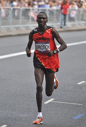 Image from Wikimedia Commons http://bit.ly/16kMKHQ Image from Wikimedia Commons http://bit.ly/16kMKHQ
|
Olympic Marathon Data
\(y = mx + c\)
\[3 = m + c\]
\[1 = 3m + c\]
\[2.5 = 2m + c\]


\(y = mx + c + \epsilon\)
\[3 = m + c + \epsilon_1\]
\[1 = 3m + c + \epsilon_2\]
\[2.5 = 2m + c + \epsilon_3\]
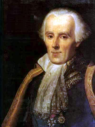
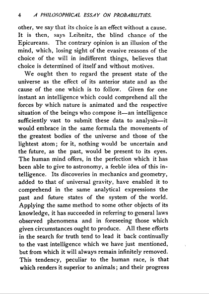
Laplace’s Idea
\[p\left(y_i|x_i\right)=\frac{1}{\sqrt{2\pi\sigma^2}}\exp \left(-\frac{\left(y_i-f\left(x_i\right)\right)^{2}}{2\sigma^2}\right).\]
Underdetermined System
- What about two unknowns and one observation? \[{y}_1 = m{x}_1 + c\]
Can compute \(m\) given \(c\). \[m = \frac{{y}_1 -c}{{x}}\]
Underdetermined System
Underdetermined System
Underdetermined System
Underdetermined System
Underdetermined System
Underdetermined System
Underdetermined System
Underdetermined System
Underdetermined System
Underdetermined System
Underdetermined System
Probability for Under- and Overdetermined
- To deal with overdetermined introduced probability distribution for ‘variable’, \({\epsilon}_i\).
- For underdetermined system introduced probability distribution for ‘parameter’, \(c\).
- This is known as a Bayesian treatment.
Bayesian Regression
Prior Distribution
Bayesian inference requires a prior on the parameters.
The prior represents your belief before you see the data of the likely value of the parameters.
For linear regression, consider a Gaussian prior on the intercept: \[c \sim {\mathcal{N}\left(0,\alpha_1\right)}\]
Posterior Distribution
Posterior distribution is found by combining the prior with the likelihood.
Posterior distribution is your belief after you see the data of the likely value of the parameters.
The posterior is found through Bayes’ Rule \[p(c|{y}) = \frac{p({y}|c)p(c)}{p({y})}\]
Bayes Update
Bayes Update
Bayes Update
Stages to Derivation of the Posterior
Multiply likelihood by prior
- they are “exponentiated quadratics”, the answer is always also an exponentiated quadratic because \(\exp(a^2)\exp(b^2) = \exp(a^2 + b^2)\).
Complete the square to get the resulting density in the form of a Gaussian.
Recognise the mean and (co)variance of the Gaussian. This is the estimate of the posterior.
Multivariate Analysis
- For general Bayesian inference need multivariate priors.
- E.g. for multivariate linear regression:
\[{y}_i = \sum_i {w}_j {x}_{i, j} + {\epsilon}_i\]
\[{y}_i = {\mathbf{{w}}}^\top {{\bf {x}}}_{i, :} + {\epsilon}_i\]
(where we’ve dropped \(c\) for convenience), we need a prior over \({\mathbf{{w}}}\).
- This motivates a multivariate Gaussian density.
- We will use the multivariate Gaussian to put a prior directly on the function (a Gaussian process).
Multivariate Bayesian Regression
Multivariate Regression Likelihood
- Noise corrupted data point \[{y}_i = {{\mathbf{{w}}}}^\top {{\bf {x}}}_{i, :} + {{\epsilon}}_i\]
- Multivariate regression likelihood: \[p({\mathbf{{y}}}| {{\bf X}}, {{\mathbf{{w}}}}) = \frac{1}{\left(2\pi {{\sigma}}^2\right)^{{{n}}/2}} \exp\left(-\frac{1}{2{{\sigma}}^2}\sum_{i=1}^{{n}}\left({y}_i - {{\mathbf{{w}}}}^\top {{\bf {x}}}_{i, :}\right)^2\right)\]
- Now use a multivariate Gaussian prior: \[p({{\mathbf{{w}}}}) = \frac{1}{\left(2\pi \alpha\right)^\frac{{p}}{2}} \exp \left(-\frac{1}{2\alpha} {{\mathbf{{w}}}}^\top {{\mathbf{{w}}}}\right)\]
Two Dimensional Gaussian Distribution
Two Dimensional Gaussian
Consider height, \(h/m\) and weight, \(w/kg\).
Could sample height from a distribution: \[p(h) \sim {\mathcal{N}\left(1.7,0.0225\right)}\]
And similarly weight: \[p(w) \sim {\mathcal{N}\left(75,36\right)}\]
Height and Weight Models
Gaussian distributions for height and weight.
Sampling Two Dimensional Variables
Independent samples of height and weight
Sampling Two Dimensional Variables
Independent samples of height and weight
Sampling Two Dimensional Variables
Independent samples of height and weight
Sampling Two Dimensional Variables
Independent samples of height and weight
Sampling Two Dimensional Variables
Independent samples of height and weight
Sampling Two Dimensional Variables
Independent samples of height and weight
Sampling Two Dimensional Variables
Independent samples of height and weight
Sampling Two Dimensional Variables
Independent samples of height and weight
Independence Assumption
This assumes height and weight are independent. \[p(h, w) = p(h)p(w)\]
In reality they are dependent (body mass index) \(= \frac{w}{h^2}\).
Sampling Two Dimensional Variables
Correlated samples of height and weight
Sampling Two Dimensional Variables
Correlated samples of height and weight
Sampling Two Dimensional Variables
Correlated samples of height and weight
Sampling Two Dimensional Variables
Correlated samples of height and weight
Sampling Two Dimensional Variables
Correlated samples of height and weight
Sampling Two Dimensional Variables
Correlated samples of height and weight
Sampling Two Dimensional Variables
Correlated samples of height and weight
Sampling Two Dimensional Variables
Correlated samples of height and weight
Independent Gaussians
\[ p(w, h) = p(w)p(h) \]
Independent Gaussians
\[ p(w, h) = \frac{1}{\sqrt{2\pi {\sigma}_1^2}\sqrt{2\pi{\sigma}_2^2}} \exp\left(-\frac{1}{2}\left(\frac{(w-{\mu}_1)^2}{{\sigma}_1^2} + \frac{(h-{\mu}_2)^2}{{\sigma}_2^2}\right)\right) \]
Independent Gaussians
\[ p(w, h) = \frac{1}{\sqrt{2\pi{\sigma}_1^22\pi{\sigma}_2^2}} \exp\left(-\frac{1}{2}\left(\begin{bmatrix}w \\ h\end{bmatrix} - \begin{bmatrix}{\mu}_1 \\ {\mu}_2\end{bmatrix}\right)^\top\begin{bmatrix}{\sigma}_1^2& 0\\0&{\sigma}_2^2\end{bmatrix}^{-1}\left(\begin{bmatrix}w \\ h\end{bmatrix} - \begin{bmatrix}{\mu}_1 \\ {\mu}_2\end{bmatrix}\right)\right) \]
Independent Gaussians
\[ p({\mathbf{{y}}}) = \frac{1}{{\left|2\pi \mathbf{D}\right|}^{\frac{1}{2}}} \exp\left(-\frac{1}{2}({\mathbf{{y}}}- {\boldsymbol{{\mu}}})^\top\mathbf{D}^{-1}({\mathbf{{y}}}- {\boldsymbol{{\mu}}})\right) \]
Correlated Gaussian
Form correlated from original by rotating the data space using matrix \({\mathbf{R}}\).
\[ p({\mathbf{{y}}}) = \frac{1}{{\left|2\pi\mathbf{D}\right|}^{\frac{1}{2}}} \exp\left(-\frac{1}{2}({\mathbf{{y}}}- {\boldsymbol{{\mu}}})^\top\mathbf{D}^{-1}({\mathbf{{y}}}- {\boldsymbol{{\mu}}})\right) \]
Correlated Gaussian
Form correlated from original by rotating the data space using matrix \({\mathbf{R}}\).
\[ p({\mathbf{{y}}}) = \frac{1}{{\left|2\pi\mathbf{D}\right|}^{\frac{1}{2}}} \exp\left(-\frac{1}{2}({\mathbf{R}}^\top{\mathbf{{y}}}- {\mathbf{R}}^\top{\boldsymbol{{\mu}}})^\top\mathbf{D}^{-1}({\mathbf{R}}^\top{\mathbf{{y}}}- {\mathbf{R}}^\top{\boldsymbol{{\mu}}})\right) \]
Correlated Gaussian
Form correlated from original by rotating the data space using matrix \({\mathbf{R}}\).
\[ p({\mathbf{{y}}}) = \frac{1}{{\left|2\pi\mathbf{D}\right|}^{\frac{1}{2}}} \exp\left(-\frac{1}{2}({\mathbf{{y}}}- {\boldsymbol{{\mu}}})^\top{\mathbf{R}}\mathbf{D}^{-1}{\mathbf{R}}^\top({\mathbf{{y}}}- {\boldsymbol{{\mu}}})\right) \] this gives a covariance matrix: \[ {\mathbf{C}}^{-1} = {\mathbf{R}}\mathbf{D}^{-1} {\mathbf{R}}^\top \]
Correlated Gaussian
Form correlated from original by rotating the data space using matrix \({\mathbf{R}}\).
\[ p({\mathbf{{y}}}) = \frac{1}{{\left|2\pi{\mathbf{C}}\right|}^{\frac{1}{2}}} \exp\left(-\frac{1}{2}({\mathbf{{y}}}- {\boldsymbol{{\mu}}})^\top{\mathbf{C}}^{-1} ({\mathbf{{y}}}- {\boldsymbol{{\mu}}})\right) \] this gives a covariance matrix: \[ {\mathbf{C}}= {\mathbf{R}}\mathbf{D} {\mathbf{R}}^\top \]
Multivariate Gaussian Properties
Recall Univariate Gaussian Properties
- Sum of Gaussian variables is also Gaussian.
\[{y}_i \sim {\mathcal{N}\left({\mu}_i,\sigma_i^2\right)}\]
\[\sum_{i=1}^{{n}} {y}_i \sim {\mathcal{N}\left(\sum_{i=1}^{n}{\mu}_i,\sum_{i=1}^{n}\sigma_i^2\right)}\]
- Scaling a Gaussian leads to a Gaussian.
\[{y}\sim {\mathcal{N}\left({\mu},\sigma^2\right)}\]
\[{w}{y}\sim {\mathcal{N}\left({w}{\mu},{w}^2 \sigma^2\right)}\]
Multivariate Consequence
\[{{\bf {x}}}\sim {\mathcal{N}\left({\boldsymbol{{\mu}}},\boldsymbol{\Sigma}\right)}\]
\[{\mathbf{{y}}}= {\mathbf{W}}{{\bf {x}}}\]
\[{\mathbf{{y}}}\sim {\mathcal{N}\left({\mathbf{W}}{\boldsymbol{{\mu}}},{\mathbf{W}}\boldsymbol{\Sigma}{\mathbf{W}}^\top\right)}\]
Distributions over Functions
Sampling a Function
Multi-variate Gaussians
We will consider a Gaussian with a particular structure of covariance matrix.
Generate a single sample from this 25 dimensional Gaussian distribution, \({\mathbf{{f}}}=\left[{f}_{1},{f}_{2}\dots {f}_{25}\right]\).
We will plot these points against their index.
Gaussian Distribution Sample
A 25 dimensional correlated random variable (values ploted against index)
Gaussian Distribution Sample
A 25 dimensional correlated random variable (values ploted against index)
Gaussian Distribution Sample
A 25 dimensional correlated random variable (values ploted against index)
Gaussian Distribution Sample
A 25 dimensional correlated random variable (values ploted against index)
Gaussian Distribution Sample
A 25 dimensional correlated random variable (values ploted against index)
Gaussian Distribution Sample
A 25 dimensional correlated random variable (values ploted against index)
Gaussian Distribution Sample
A 25 dimensional correlated random variable (values ploted against index)
Gaussian Distribution Sample
A 25 dimensional correlated random variable (values ploted against index)
Gaussian Distribution Sample
A 25 dimensional correlated random variable (values ploted against index)
Prediction of \({f}_{2}\) from \({f}_{1}\)
A 25 dimensional correlated random variable (values ploted against index)
Prediction of \({f}_{2}\) from \({f}_{1}\)
A 25 dimensional correlated random variable (values ploted against index)
Prediction of \({f}_{2}\) from \({f}_{1}\)
A 25 dimensional correlated random variable (values ploted against index)
Prediction of \({f}_{2}\) from \({f}_{1}\)
A 25 dimensional correlated random variable (values ploted against index)
Prediction of \({f}_{5}\) from \({f}_{1}\)
A 25 dimensional correlated random variable (values ploted against index)
Prediction of \({f}_{5}\) from \({f}_{1}\)
A 25 dimensional correlated random variable (values ploted against index)
Prediction of \({f}_{5}\) from \({f}_{1}\)
A 25 dimensional correlated random variable (values ploted against index)
Prediction of \({f}_{5}\) from \({f}_{1}\)
A 25 dimensional correlated random variable (values ploted against index)