Introduction to Gaussian Processes

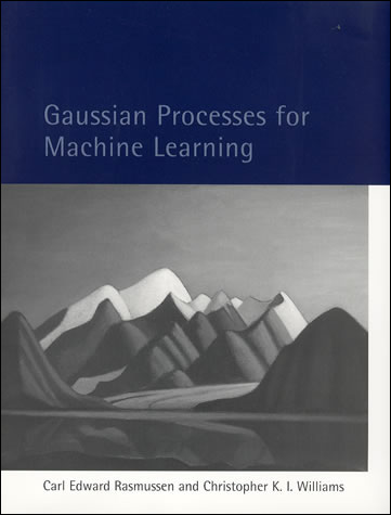
Rasmussen and Williams (2006)

What is Machine Learning?

What is Machine Learning?

\[\text{data} + \text{model} \xrightarrow{\text{compute}} \text{prediction}\]

• To combine data with a model need:
• a prediction function \(\mappingFunction(\cdot)\) includes our beliefs about the regularities of the universe
• an objective function \(\errorFunction(\cdot)\) defines the cost of misprediction.

Olympic Marathon Data

Gold medal times for Olympic Marathon since 1896. Marathons before 1924 didn’t have a standardised distance. Present results using pace per km. In 1904 Marathon was badly organised leading to very slow times.

Image from Wikimedia Commons http://bit.ly/16kMKHQ

Olympic Marathon Data

Overdetermined System

\(\dataScalar = m\inputScalar + c\)

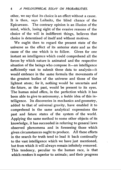
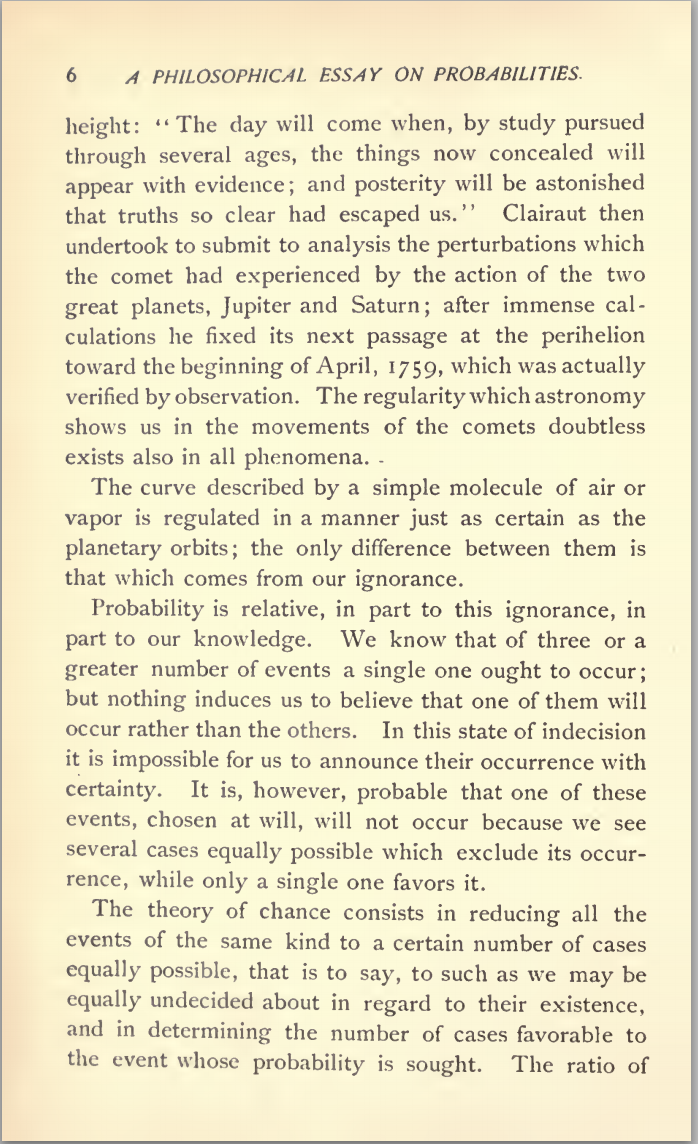
\(\dataScalar = m\inputScalar + c + \noiseScalar\)

A Probabilistic Process

The Gaussian Density

• Perhaps the most common probability density.

Gaussian Density

Gaussian Density

\[ \gaussianDist{\dataScalar}{\meanScalar}{\dataStd^2} = \frac{1}{\sqrt{2\pi\dataStd^2}} \exp\left(-\frac{(\dataScalar-\meanScalar)^2}{2\dataStd^2}\right) \]

Two Important Gaussian Properties

Sum of Gaussians

Scaling a Gaussian

Regression Examples

• Predict a real value, \(\dataScalar_i\) given some inputs \(\inputVector_i\).
• Predict quality of meat given spectral measurements (Tecator data).
• Radiocarbon dating, the C14 calibration curve: predict age given quantity of C14 isotope.
• Predict quality of different Go or Backgammon moves given expert rated training data.

Underdetermined System

• What about two unknowns and one observation? \[\dataScalar_1 = m\inputScalar_1 + c\]

Underdetermined System

Overdetermined System

• With two unknowns and two observations: \[\begin{aligned} \dataScalar_1 = & m\inputScalar_1 + c\\ \dataScalar_2 = & m\inputScalar_2 + c \end{aligned}\]

• Additional observation leads to overdetermined system. \[\dataScalar_3 = m\inputScalar_3 + c\]

Overdetermined System

• This problem is solved through a noise model \(\noiseScalar \sim \gaussianSamp{0}{\dataStd^2}\) \[\begin{aligned} \dataScalar_1 = m\inputScalar_1 + c + \noiseScalar_1\\ \dataScalar_2 = m\inputScalar_2 + c + \noiseScalar_2\\ \dataScalar_3 = m\inputScalar_3 + c + \noiseScalar_3 \end{aligned}\]

Noise Models

• We aren’t modeling entire system.
• Noise model gives mismatch between model and data.
• Gaussian model justified by appeal to central limit theorem.
• Other models also possible (Student-\(t\) for heavy tails).
• Maximum likelihood with Gaussian noise leads to least squares.

Probability for Under- and Overdetermined

• To deal with overdetermined introduced probability distribution for ‘variable’, \({\noiseScalar}_i\).

Different Types of Uncertainty

• The first type of uncertainty we are assuming is aleatoric uncertainty.
• The second type of uncertainty we are assuming is epistemic uncertainty.

Aleatoric Uncertainty

• This is uncertainty we couldn’t know even if we wanted to. e.g. the result of a football match before it’s played.
• Where a sheet of paper might land on the floor.

Epistemic Uncertainty

• This is uncertainty we could in principle know the answer too. We just haven’t observed enough yet, e.g. the result of a football match after it’s played.
• What colour socks your lecturer is wearing.

Bayesian Regression

Prior Distribution

• Bayesian inference requires a prior on the parameters.
• The prior represents your belief before you see the data of the likely value of the parameters.
• For linear regression, consider a Gaussian prior on the intercept:

\[c \sim \gaussianSamp{0}{\alpha_1}\]

Posterior Distribution

• Posterior distribution is found by combining the prior with the likelihood.
• Posterior distribution is your belief after you see the data of the likely value of the parameters.
• The posterior is found through Bayes’ Rule \[ p(c|\dataScalar) = \frac{p(\dataScalar|c)p(c)}{p(\dataScalar)} \]

\[ \text{posterior} = \frac{\text{likelihood}\times \text{prior}}{\text{marginal likelihood}}. \]

Bayes Update

Stages to Derivation of the Posterior

• Multiply likelihood by prior
• they are “exponentiated quadratics”, the answer is always also an exponentiated quadratic because \(\exp(a^2)\exp(b^2) = \exp(a^2 + b^2)\).
• Complete the square to get the resulting density in the form of a Gaussian.
• Recognise the mean and (co)variance of the Gaussian. This is the estimate of the posterior.

Multivariate System

• For general Bayesian inference need multivariate priors.

Multivariate System

• This motivates a multivariate Gaussian density.

Multivariate Bayesian Regression

Multivariate Regression Likelihood

• Noise corrupted data point \[\dataScalar_i = \weightVector^\top \inputVector_{i, :} + {\noiseScalar}_i\]

Two Dimensional Gaussian Distribution

Two Dimensional Gaussian

• Consider height, \(h/m\) and weight, \(w/kg\).
• Could sample height from a distribution: \[ p(h) \sim \gaussianSamp{1.7}{0.0225}. \]
• And similarly weight: \[ p(w) \sim \gaussianSamp{75}{36}. \]

Height and Weight Models

Independence Assumption

• We assume height and weight are independent.

\[ p(w, h) = p(w)p(h). \]

Sampling Two Dimensional Variables

Body Mass Index

• In reality they are dependent (body mass index) \(= \frac{w}{h^2}\).
• To deal with this dependence we introduce correlated multivariate Gaussians.

Sampling Two Dimensional Variables

Independent Gaussians

\[ p(w, h) = p(w)p(h) \]

Independent Gaussians

\[ p(w, h) = \frac{1}{\sqrt{2\pi \dataStd_1^2}\sqrt{2\pi\dataStd_2^2}} \exp\left(-\frac{1}{2}\left(\frac{(w-\meanScalar_1)^2}{\dataStd_1^2} + \frac{(h-\meanScalar_2)^2}{\dataStd_2^2}\right)\right) \]

Independent Gaussians

\[ p(w, h) = \frac{1}{\sqrt{2\pi\dataStd_1^22\pi\dataStd_2^2}} \exp\left(-\frac{1}{2}\left(\begin{bmatrix}w \\ h\end{bmatrix} - \begin{bmatrix}\meanScalar_1 \\ \meanScalar_2\end{bmatrix}\right)^\top\begin{bmatrix}\dataStd_1^2& 0\\0&\dataStd_2^2\end{bmatrix}^{-1}\left(\begin{bmatrix}w \\ h\end{bmatrix} - \begin{bmatrix}\meanScalar_1 \\ \meanScalar_2\end{bmatrix}\right)\right) \]

Independent Gaussians

\[ p(\dataVector) = \frac{1}{\det{2\pi \mathbf{D}}^{\frac{1}{2}}} \exp\left(-\frac{1}{2}(\dataVector - \meanVector)^\top\mathbf{D}^{-1}(\dataVector - \meanVector)\right) \]

Correlated Gaussian

Form correlated from original by rotating the data space using matrix \(\rotationMatrix\).

\[ p(\dataVector) = \frac{1}{\det{2\pi\mathbf{D}}^{\frac{1}{2}}} \exp\left(-\frac{1}{2}(\dataVector - \meanVector)^\top\mathbf{D}^{-1}(\dataVector - \meanVector)\right) \]

Correlated Gaussian

Form correlated from original by rotating the data space using matrix \(\rotationMatrix\).

\[ p(\dataVector) = \frac{1}{\det{2\pi\mathbf{D}}^{\frac{1}{2}}} \exp\left(-\frac{1}{2}(\rotationMatrix^\top\dataVector - \rotationMatrix^\top\meanVector)^\top\mathbf{D}^{-1}(\rotationMatrix^\top\dataVector - \rotationMatrix^\top\meanVector)\right) \]

Correlated Gaussian

Form correlated from original by rotating the data space using matrix \(\rotationMatrix\).

\[ p(\dataVector) = \frac{1}{\det{2\pi\mathbf{D}}^{\frac{1}{2}}} \exp\left(-\frac{1}{2}(\dataVector - \meanVector)^\top\rotationMatrix\mathbf{D}^{-1}\rotationMatrix^\top(\dataVector - \meanVector)\right) \] this gives a covariance matrix: \[ \covarianceMatrix^{-1} = \rotationMatrix \mathbf{D}^{-1} \rotationMatrix^\top \]

Correlated Gaussian

Form correlated from original by rotating the data space using matrix \(\rotationMatrix\).

\[ p(\dataVector) = \frac{1}{\det{2\pi\covarianceMatrix}^{\frac{1}{2}}} \exp\left(-\frac{1}{2}(\dataVector - \meanVector)^\top\covarianceMatrix^{-1} (\dataVector - \meanVector)\right) \] this gives a covariance matrix: \[ \covarianceMatrix = \rotationMatrix \mathbf{D} \rotationMatrix^\top \]

Multivariate Gaussian Properties

Recall Univariate Gaussian Properties

Recall Univariate Gaussian Properties

2. Scaling a Gaussian leads to a Gaussian.

Multivariate Consequence

If \[\inputVector \sim \gaussianSamp{\meanVector}{\covarianceMatrix}\]

Linear Gaussian Models

Gaussian processes are initially of interest because 1. linear Gaussian models are easier to deal with 2. Even the parameters within the process can be handled, by considering a particular limit.

Multivariate Gaussian Properties

• If \[ \dataVector = \mappingMatrix \inputVector + \noiseVector, \]

• Assume \[\begin{align} \inputVector & \sim \gaussianSamp{\meanVector}{\covarianceMatrix}\\ \noiseVector & \sim \gaussianSamp{\zerosVector}{\covarianceMatrixTwo} \end{align}\]

• Then \[ \dataVector \sim \gaussianSamp{\mappingMatrix\meanVector}{\mappingMatrix\covarianceMatrix\mappingMatrix^\top + \covarianceMatrixTwo}. \] If \(\covarianceMatrixTwo=\dataStd^2\eye\), this is Probabilistic Principal Component Analysis (Tipping and Bishop, 1999), because we integrated out the inputs (or latent variables they would be called in that case).

Non linear on Inputs

• Set each activation function computed at each data point to be

\[ \activationScalar_{i,j} = \activationScalar(\mappingVector^{(1)}_{j}, \inputVector_{i}) \] Define design matrix \[ \activationMatrix = \begin{bmatrix} \activationScalar_{1, 1} & \activationScalar_{1, 2} & \dots & \activationScalar_{1, \numHidden} \\ \activationScalar_{1, 2} & \activationScalar_{1, 2} & \dots & \activationScalar_{1, \numData} \\ \vdots & \vdots & \ddots & \vdots \\ \activationScalar_{\numData, 1} & \activationScalar_{\numData, 2} & \dots & \activationScalar_{\numData, \numHidden} \end{bmatrix}. \]

Matrix Representation of a Neural Network

\[\dataScalar\left(\inputVector\right) = \activationVector\left(\inputVector\right)^\top \mappingVector + \noiseScalar\]

Prior Density

• Define

\[ \mappingVector \sim \gaussianSamp{\zerosVector}{\alpha\eye}, \]

• Rules of multivariate Gaussians to see that,

\[ \dataVector \sim \gaussianSamp{\zerosVector}{\alpha \activationMatrix \activationMatrix^\top + \dataStd^2 \eye}. \]

\[ \kernelMatrix = \alpha \activationMatrix \activationMatrix^\top + \dataStd^2 \eye. \]

Joint Gaussian Density

• Elements are a function \(\kernel_{i,j} = \kernel\left(\inputVector_i, \inputVector_j\right)\)

\[ \kernelMatrix = \alpha \activationMatrix \activationMatrix^\top + \dataStd^2 \eye. \]

Covariance Function

\[ \kernel_\mappingFunction\left(\inputVector_i, \inputVector_j\right) = \alpha \activationVector\left(\mappingMatrix_1, \inputVector_i\right)^\top \activationVector\left(\mappingMatrix_1, \inputVector_j\right) \]

• formed by inner products of the rows of the design matrix.

Gaussian Process

• Instead of making assumptions about our density over each data point, \(\dataScalar_i\) as i.i.d.

• make a joint Gaussian assumption over our data.

• covariance matrix is now a function of both the parameters of the activation function, \(\mappingMatrix_1\), and the input variables, \(\inputMatrix\).

• Arises from integrating out \(\mappingVector^{(2)}\).

Basis Functions

• Can be very complex, such as deep kernels, (Cho and Saul, 2009) or could even put a convolutional neural network inside.
• Viewing a neural network in this way is also what allows us to beform sensible batch normalizations (Ioffe and Szegedy, 2015).

Distributions over Functions

Sampling a Function

Multi-variate Gaussians

• We will consider a Gaussian with a particular structure of covariance matrix.
• Generate a single sample from this 25 dimensional Gaussian density, \[ \mappingFunctionVector=\left[\mappingFunction_{1},\mappingFunction_{2}\dots \mappingFunction_{25}\right]. \]
• We will plot these points against their index.

Gaussian Distribution Sample

Prediction of \(\mappingFunction_{2}\) from \(\mappingFunction_{1}\)

Uluru

Prediction with Correlated Gaussians

• Prediction of \(\mappingFunction_2\) from \(\mappingFunction_1\) requires conditional density.
• Conditional density is also Gaussian. \[ p(\mappingFunction_2|\mappingFunction_1) = \gaussianDist{\mappingFunction_2}{\frac{\kernelScalar_{1, 2}}{\kernelScalar_{1, 1}}\mappingFunction_1}{ \kernelScalar_{2, 2} - \frac{\kernelScalar_{1,2}^2}{\kernelScalar_{1,1}}} \] where covariance of joint density is given by \[ \kernelMatrix = \begin{bmatrix} \kernelScalar_{1, 1} & \kernelScalar_{1, 2}\\ \kernelScalar_{2, 1} & \kernelScalar_{2, 2}.\end{bmatrix} \]

Prediction of \(\mappingFunction_{8}\) from \(\mappingFunction_{1}\)

Where Did This Covariance Matrix Come From?

\[ k(\inputVector, \inputVector^\prime) = \alpha \exp\left(-\frac{\left\Vert \inputVector - \inputVector^\prime\right\Vert^2_2}{2\lengthScale^2}\right)\]

Computing Covariance

Computing Covariance

Computing Covariance

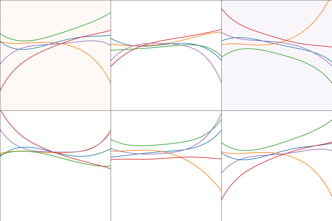
Polynomial Covariance

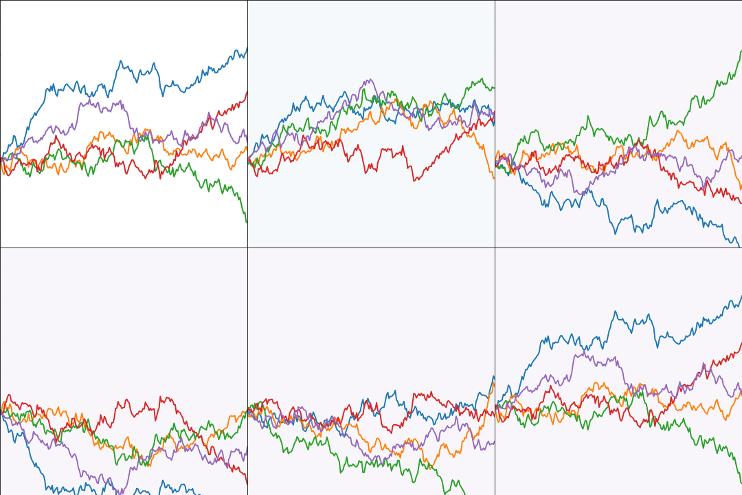
Brownian Covariance

\[ \kernelScalar(t, t^\prime) = \alpha \min(t, t^\prime) \]

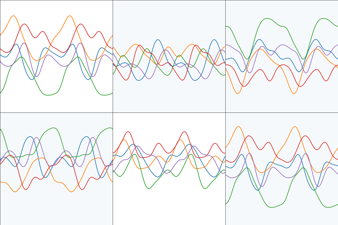
Periodic Covariance

Covariance Functions

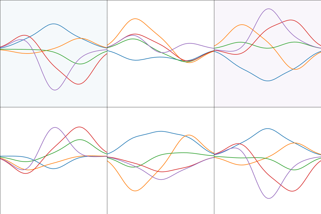
RBF Basis Functions

\[ \basisFunction_k(\inputScalar) = \exp\left(-\frac{\ltwoNorm{\inputScalar-\meanScalar_k}^{2}}{\lengthScale^{2}}\right). \]

\[ \meanVector = \begin{bmatrix} -1 \\ 0 \\ 1\end{bmatrix}, \]

\[ \kernelScalar\left(\inputVals,\inputVals^{\prime}\right)=\alpha\basisVector(\inputVals)^\top \basisVector(\inputVals^\prime). \]

Basis Function Covariance

Selecting Number and Location of Basis

• Need to choose

1. location of centers
2. number of basis functions Restrict analysis to 1-D input, \(\inputScalar\).

• Consider uniform spacing over a region:

Uniform Basis Functions

• Set each center location to \[\locationScalar_k = a+\Delta\locationScalar\cdot (k-1).\]

• Specify the basis functions in terms of their indices, \[\begin{aligned} \kernelScalar\left(\inputScalar_i,\inputScalar_j\right) = &\alpha^\prime\Delta\locationScalar \sum_{k=1}^{\numBasisFunc} \exp\Bigg( -\frac{\inputScalar_i^2 + \inputScalar_j^2}{2\rbfWidth^2}\\ & - \frac{2\left(a+\Delta\locationScalar\cdot (k-1)\right) \left(\inputScalar_i+\inputScalar_j\right) + 2\left(a+\Delta\locationScalar \cdot (k-1)\right)^2}{2\rbfWidth^2} \Bigg) \end{aligned}\]

where we’ve scaled variance of process by \(\Delta\locationScalar\).

Infinite Basis Functions

• Take \[ \locationScalar_1=a \ \text{and}\ \locationScalar_\numBasisFunc=b \ \text{so}\ b= a+ \Delta\locationScalar\cdot(\numBasisFunc-1) \]

• This implies \[ b-a = \Delta\locationScalar (\numBasisFunc -1) \] and therefore \[ \numBasisFunc = \frac{b-a}{\Delta \locationScalar} + 1 \]

• Take limit as \(\Delta\locationScalar\rightarrow 0\) so \(\numBasisFunc \rightarrow \infty\) where we have used \(a + k\cdot\Delta\locationScalar\rightarrow \locationScalar\).

Result

• Performing the integration leads to \[\begin{aligned} \kernelScalar(\inputScalar_i,&\inputScalar_j) = \alpha^\prime \sqrt{\pi\rbfWidth^2} \exp\left( -\frac{\left(\inputScalar_i-\inputScalar_j\right)^2}{4\rbfWidth^2}\right)\\ &\times \frac{1}{2}\left[\text{erf}\left(\frac{\left(b - \frac{1}{2}\left(\inputScalar_i + \inputScalar_j\right)\right)}{\rbfWidth} \right)- \text{erf}\left(\frac{\left(a - \frac{1}{2}\left(\inputScalar_i + \inputScalar_j\right)\right)}{\rbfWidth} \right)\right], \end{aligned}\]
• Now take limit as \(a\rightarrow -\infty\) and \(b\rightarrow \infty\) \[\kernelScalar\left(\inputScalar_i,\inputScalar_j\right) = \alpha\exp\left( -\frac{\left(\inputScalar_i-\inputScalar_j\right)^2}{4\rbfWidth^2}\right).\] where \(\alpha=\alpha^\prime \sqrt{\pi\rbfWidth^2}\).

Infinite Feature Space

• An RBF model with infinite basis functions is a Gaussian process.
• The covariance function is given by the  covariance function. \[\kernelScalar\left(\inputScalar_i,\inputScalar_j\right) = \alpha \exp\left( -\frac{\left(\inputScalar_i-\inputScalar_j\right)^2}{4\rbfWidth^2}\right).\]

Infinite Feature Space

• An RBF model with infinite basis functions is a Gaussian process.
• The covariance function is the exponentiated quadratic (squared exponential).
• Note: The functional form for the covariance function and basis functions are similar.
• this is a special case,
• in general they are very different

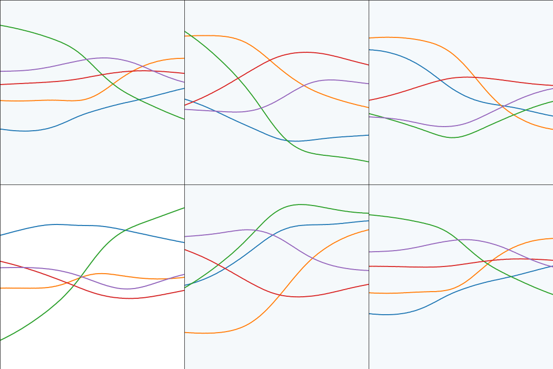
MLP Covariance

Sinc Covariance

References

Cho, Y., Saul, L.K., 2009. Kernel methods for deep learning, in: Bengio, Y., Schuurmans, D., Lafferty, J.D., Williams, C.K.I., Culotta, A. (Eds.), Advances in Neural Information Processing Systems 22. Curran Associates, Inc., pp. 342–350.
Ioffe, S., Szegedy, C., 2015. Batch normalization: Accelerating deep network training by reducing internal covariate shift, in: Bach, F., Blei, D. (Eds.), Proceedings of the 32nd International Conference on Machine Learning, Proceedings of Machine Learning Research. PMLR, Lille, France, pp. 448–456.
Rasmussen, C.E., Williams, C.K.I., 2006. Gaussian processes for machine learning. mit, Cambridge, MA.
Tipping, M.E., Bishop, C.M., 1999. Probabilistic principal component analysis. Journal of the Royal Statistical Society, B 6, 611–622. https://doi.org/doi:10.1111/1467-9868.00196