Gaussian Processes

What is Machine Learning?

What is Machine Learning?

\[\text{data} + \text{model} \xrightarrow{\text{compute}} \text{prediction}\]

• To combine data with a model need:
• a prediction function \(\mappingFunction(\cdot)\) includes our beliefs about the regularities of the universe
• an objective function \(\errorFunction(\cdot)\) defines the cost of misprediction.

Artificial Intelligence

• Machine learning is a mainstay because of importance of prediction.

Uncertainty

• Uncertainty in prediction arises from:
• scarcity of training data and
• mismatch between the set of prediction functions we choose and all possible prediction functions.
• Also uncertainties in objective, leave those for another day.

Neural Networks and Prediction Functions

• adaptive non-linear function models inspired by simple neuron models (McCulloch and Pitts, 1943)
• have become popular because of their ability to model data.
• can be composed to form highly complex functions
• start by focussing on one hidden layer

Prediction Function of One Hidden Layer

\[ \mappingFunction(\inputVector) = \left.\mappingVector^{(2)}\right.^\top \activationVector(\mappingMatrix_{1}, \inputVector) \]

\(\mappingFunction(\cdot)\) is a scalar function with vector inputs,

\(\activationVector(\cdot)\) is a vector function with vector inputs.

• dimensionality of the vector function is known as the number of hidden units, or the number of neurons.

• elements of \(\activationVector(\cdot)\) are the activation function of the neural network

• elements of \(\mappingMatrix_{1}\) are the parameters of the activation functions.

Relations with Classical Statistics

• In statistics activation functions are known as basis functions.

• would think of this as a linear model: not linear predictions, linear in the parameters

• \(\mappingVector_{1}\) are static parameters.

Adaptive Basis Functions

• In machine learning we optimize \(\mappingMatrix_{1}\) as well as \(\mappingMatrix_{2}\) (which would normally be denoted in statistics by \(\boldsymbol{\beta}\)).

• Revisit that decision: follow the path of Neal (1994) and MacKay (1992).

• Consider the probabilistic approach.

Probabilistic Modelling

• Probabilistically we want, \[ p(\dataScalar_*|\dataVector, \inputMatrix, \inputVector_*), \] \(\dataScalar_*\) is a test output \(\inputVector_*\) is a test input \(\inputMatrix\) is a training input matrix \(\dataVector\) is training outputs

Joint Model of World

\[ p(\dataScalar_*|\dataVector, \inputMatrix, \inputVector_*) = \int p(\dataScalar_*|\inputVector_*, \mappingMatrix) p(\mappingMatrix | \dataVector, \inputMatrix) \text{d} \mappingMatrix \]

Likelihood

\(p(\dataScalar|\inputVector, \mappingMatrix)\) is the likelihood of data point

Likelihood and Prediction Function

\[ p(\dataScalar_i | \mappingFunction(\inputVector_i)) = \frac{1}{\sqrt{2\pi \dataStd^2}} \exp\left(-\frac{\left(\dataScalar_i - \mappingFunction(\inputVector_i)\right)^2}{2\dataStd^2}\right) \]

Unsupervised Learning

• Can also consider priors over latents \[ p(\dataVector_*|\dataVector) = \int p(\dataVector_*|\inputMatrix_*, \mappingMatrix) p(\mappingMatrix | \dataVector, \inputMatrix) p(\inputMatrix) p(\inputMatrix_*) \text{d} \mappingMatrix \text{d} \inputMatrix \text{d}\inputMatrix_* \]

• This gives unsupervised learning.

Probabilistic Inference

• Data: \(\dataVector\)

• Model: \(p(\dataVector, \dataVector^*)\)

• Prediction: \(p(\dataVector^*| \dataVector)\)

Graphical Models

• Represent joint distribution through conditional dependencies.
• E.g. Markov chain

\[p(\dataVector) = p(\dataScalar_\numData | \dataScalar_{\numData-1}) p(\dataScalar_{\numData-1}|\dataScalar_{\numData-2}) \dots p(\dataScalar_{2} | \dataScalar_{1})\]

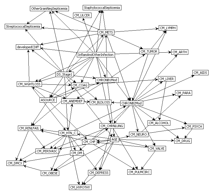
Predict Perioperative Risk of Clostridium Difficile Infection Following Colon Surgery (Steele et al., 2012)

Performing Inference

• Easy to write in probabilities

• But underlying this is a wealth of computational challenges.

• High dimensional integrals typically require approximation.

Linear Models

• In statistics, focussed more on linear model implied by \[ \mappingFunction(\inputVector) = \left.\mappingVector^{(2)}\right.^\top \activationVector(\mappingMatrix_1, \inputVector) \]

• Hold \(\mappingMatrix_1\) fixed for given analysis.

• Gaussian prior for \(\mappingMatrix\), \[ \mappingVector^{(2)} \sim \gaussianSamp{\zerosVector}{\covarianceMatrix}. \] \[ \dataScalar_i = \mappingFunction(\inputVector_i) + \noiseScalar_i, \] where \[ \noiseScalar_i \sim \gaussianSamp{0}{\dataStd^2} \]

Linear Gaussian Models

• Normally integrals are complex but for this Gaussian linear case they are trivial.

Multivariate Gaussian Properties

Recall Univariate Gaussian Properties

Recall Univariate Gaussian Properties

2. Scaling a Gaussian leads to a Gaussian.

Multivariate Consequence

If \[\inputVector \sim \gaussianSamp{\meanVector}{\covarianceMatrix}\]

Linear Gaussian Models

1. linear Gaussian models are easier to deal with
2. Even the parameters within the process can be handled, by considering a particular limit.

Multivariate Gaussian Properties

• If \[ \dataVector = \mappingMatrix \inputVector + \noiseVector, \]

• Assume \[ \begin{align} \inputVector & \sim \gaussianSamp{\meanVector}{\covarianceMatrix}\\ \noiseVector & \sim \gaussianSamp{\zerosVector}{\covarianceMatrixTwo} \end{align} \]

• Then \[ \dataVector \sim \gaussianSamp{\mappingMatrix\meanVector}{\mappingMatrix\covarianceMatrix\mappingMatrix^\top + \covarianceMatrixTwo}. \] If \(\covarianceMatrixTwo=\dataStd^2\eye\), this is Probabilistic Principal Component Analysis (Tipping and Bishop, 1999), because we integrated out the inputs (or latent variables they would be called in that case).

Non linear on Inputs

• Set each activation function computed at each data point to be

\[ \activationScalar_{i,j} = \activationScalar(\mappingVector^{(1)}_{j}, \inputVector_{i}) \] Define design matrix \[ \activationMatrix = \begin{bmatrix} \activationScalar_{1, 1} & \activationScalar_{1, 2} & \dots & \activationScalar_{1, \numHidden} \\ \activationScalar_{1, 2} & \activationScalar_{1, 2} & \dots & \activationScalar_{1, \numData} \\ \vdots & \vdots & \ddots & \vdots \\ \activationScalar_{\numData, 1} & \activationScalar_{\numData, 2} & \dots & \activationScalar_{\numData, \numHidden} \end{bmatrix}. \]

Matrix Representation of a Neural Network

\[\dataScalar\left(\inputVector\right) = \activationVector\left(\inputVector\right)^\top \mappingVector + \noiseScalar\]

Prior Density

• Define

\[ \mappingVector \sim \gaussianSamp{\zerosVector}{\alpha\eye}, \]

• Rules of multivariate Gaussians to see that,

\[ \dataVector \sim \gaussianSamp{\zerosVector}{\alpha \activationMatrix \activationMatrix^\top + \dataStd^2 \eye}. \]

\[ \kernelMatrix = \alpha \activationMatrix \activationMatrix^\top + \dataStd^2 \eye. \]

Joint Gaussian Density

• Elements are a function \(\kernel_{i,j} = \kernel\left(\inputVector_i, \inputVector_j\right)\)

\[ \kernelMatrix = \alpha \activationMatrix \activationMatrix^\top + \dataStd^2 \eye. \]

Covariance Function

\[ \kernel_\mappingFunction\left(\inputVector_i, \inputVector_j\right) = \alpha \activationVector\left(\mappingMatrix_1, \inputVector_i\right)^\top \activationVector\left(\mappingMatrix_1, \inputVector_j\right) \]

• formed by inner products of the rows of the design matrix.

Gaussian Process

• Instead of making assumptions about our density over each data point, \(\dataScalar_i\) as i.i.d.

• make a joint Gaussian assumption over our data.

• covariance matrix is now a function of both the parameters of the activation function, \(\mappingMatrix_1\), and the input variables, \(\inputMatrix\).

• Arises from integrating out \(\mappingVector^{(2)}\).

Basis Functions

• Can be very complex, such as deep kernels, (Cho and Saul, 2009) or could even put a convolutional neural network inside.
• Viewing a neural network in this way is also what allows us to beform sensible batch normalizations (Ioffe and Szegedy, 2015).

Non-degenerate Gaussian Processes

• This process is degenerate.
• Covariance function is of rank at most \(\numHidden\).
• As \(\numData \rightarrow \infty\), covariance matrix is not full rank.
• Leading to \(\det{\kernelMatrix} = 0\)

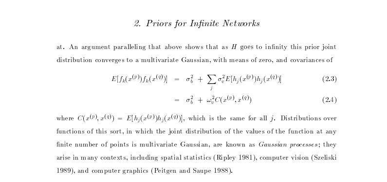
Infinite Networks

• In ML Radford Neal (Neal, 1994) asked “what would happen if you took \(\numHidden \rightarrow \infty\)?”

Roughly Speaking

• Instead of

\[ \begin{align*} \kernel_\mappingFunction\left(\inputVector_i, \inputVector_j\right) & = \alpha \activationVector\left(\mappingMatrix_1, \inputVector_i\right)^\top \activationVector\left(\mappingMatrix_1, \inputVector_j\right)\\ & = \alpha \sum_k \activationScalar\left(\mappingVector^{(1)}_k, \inputVector_i\right) \activationScalar\left(\mappingVector^{(1)}_k, \inputVector_j\right) \end{align*} \]

• Sample infinitely many from a prior density, \(p(\mappingVector^{(1)})\),

\[ \kernel_\mappingFunction\left(\inputVector_i, \inputVector_j\right) = \alpha \int \activationScalar\left(\mappingVector^{(1)}, \inputVector_i\right) \activationScalar\left(\mappingVector^{(1)}, \inputVector_j\right) p(\mappingVector^{(1)}) \text{d}\mappingVector^{(1)} \]

• Also applies for non-Gaussian \(p(\mappingVector^{(1)})\) because of the central limit theorem.

Simple Probabilistic Program

• If \[ \begin{align*} \mappingVector^{(1)} & \sim p(\cdot)\\ \phi_i & = \activationScalar\left(\mappingVector^{(1)}, \inputVector_i\right), \end{align*} \] has finite variance.

• Then taking number of hidden units to infinity, is also a Gaussian process.

Further Reading

• Chapter 2 of Neal’s thesis (Neal, 1994)

• Rest of Neal’s thesis. (Neal, 1994)

• David MacKay’s PhD thesis (MacKay, 1992)

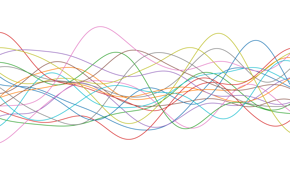
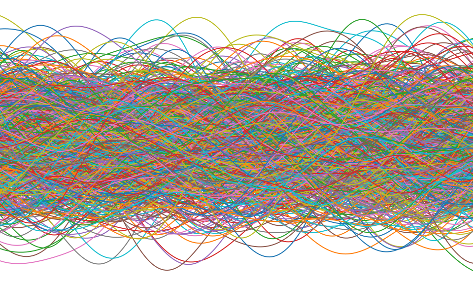
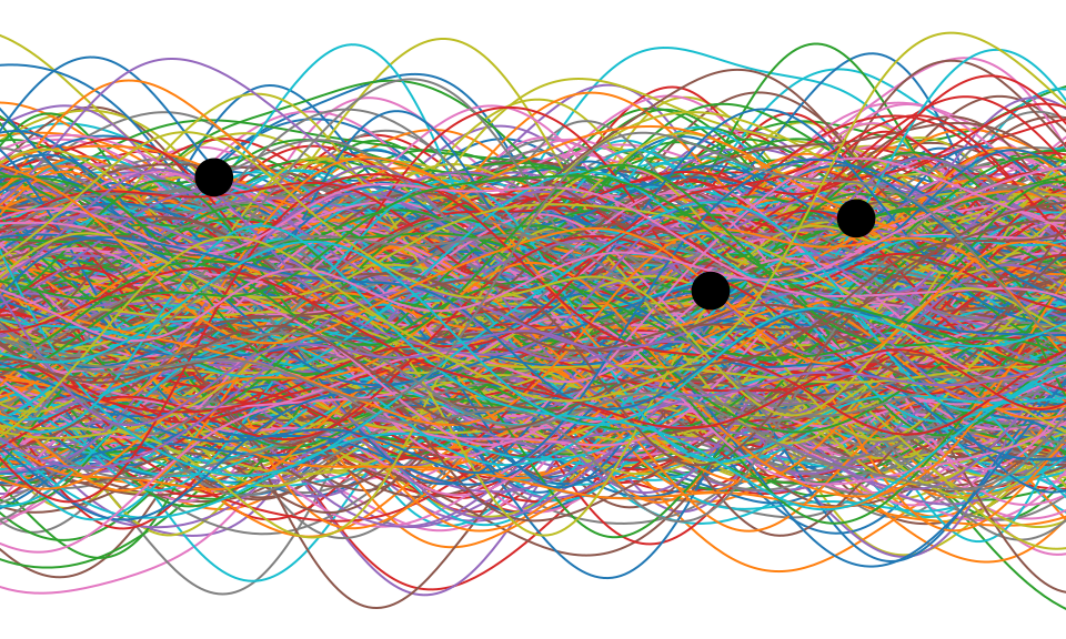
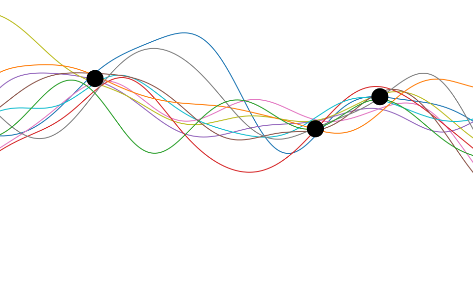
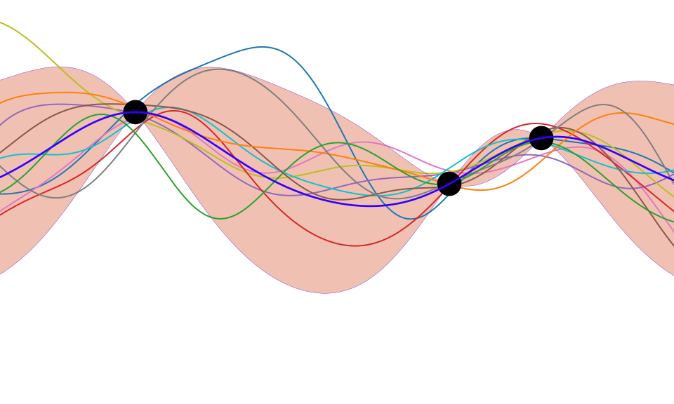
Distributions over Functions

Sampling a Function

Multi-variate Gaussians

• We will consider a Gaussian with a particular structure of covariance matrix.
• Generate a single sample from this 25 dimensional Gaussian density, \[ \mappingFunctionVector=\left[\mappingFunction_{1},\mappingFunction_{2}\dots \mappingFunction_{25}\right]. \]
• We will plot these points against their index.

Gaussian Distribution Sample

Prediction of \(\mappingFunction_{2}\) from \(\mappingFunction_{1}\)

Uluru

Prediction with Correlated Gaussians

• Prediction of \(\mappingFunction_2\) from \(\mappingFunction_1\) requires conditional density.
• Conditional density is also Gaussian. \[ p(\mappingFunction_2|\mappingFunction_1) = \gaussianDist{\mappingFunction_2}{\frac{\kernelScalar_{1, 2}}{\kernelScalar_{1, 1}}\mappingFunction_1}{ \kernelScalar_{2, 2} - \frac{\kernelScalar_{1,2}^2}{\kernelScalar_{1,1}}} \] where covariance of joint density is given by \[ \kernelMatrix = \begin{bmatrix} \kernelScalar_{1, 1} & \kernelScalar_{1, 2}\\ \kernelScalar_{2, 1} & \kernelScalar_{2, 2}.\end{bmatrix} \]

Prediction of \(\mappingFunction_{8}\) from \(\mappingFunction_{1}\)

Key Object

• Covariance function, \(\kernelMatrix\)
• Determines properties of samples.
• Function of \(\inputMatrix\), \[\kernelScalar_{i,j} = \kernelScalar(\inputVector_i, \inputVector_j)\]

Linear Algebra

• Posterior mean \[\mappingFunction_D(\inputVector_*) = \kernelVector(\inputVector_*, \inputMatrix) \kernelMatrix^{-1} \mathbf{y}\]

• Posterior covariance \[\mathbf{C}_* = \kernelMatrix_{*,*} - \kernelMatrix_{*,\mappingFunctionVector} \kernelMatrix^{-1} \kernelMatrix_{\mappingFunctionVector, *}\]

Linear Algebra

• Posterior mean

  \[\mappingFunction_D(\inputVector_*) = \kernelVector(\inputVector_*, \inputMatrix) \boldsymbol{\alpha}\]

• Posterior covariance \[\covarianceMatrix_* = \kernelMatrix_{*,*} - \kernelMatrix_{*,\mappingFunctionVector} \kernelMatrix^{-1} \kernelMatrix_{\mappingFunctionVector, *}\]

Exponentiated Quadratic Covariance

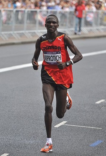
Olympic Marathon Data

Gold medal times for Olympic Marathon since 1896. Marathons before 1924 didn’t have a standardised distance. Present results using pace per km. In 1904 Marathon was badly organised leading to very slow times.

Image from Wikimedia Commons http://bit.ly/16kMKHQ

Olympic Marathon Data

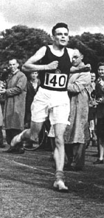
Alan Turing

Probability Winning Olympics?

• He was a formidable Marathon runner.
• In 1946 he ran a time 2 hours 46 minutes.
  • That’s a pace of 3.95 min/km.
• What is the probability he would have won an Olympics if one had been held in 1946?

Olympic Marathon Data GP

Learning Covariance Parameters

Can we determine covariance parameters from the data?

\[\gaussianDist{\dataVector}{\mathbf{0}}{\kernelMatrix}=\frac{1}{(2\pi)^\frac{\numData}{2}{\det{\kernelMatrix}^{\frac{1}{2}}}}{\exp\left(-\frac{\dataVector^{\top}\kernelMatrix^{-1}\dataVector}{2}\right)}\]

\[\begin{aligned} \gaussianDist{\dataVector}{\mathbf{0}}{\kernelMatrix}=\frac{1}{(2\pi)^\frac{\numData}{2}{\color{white} \det{\kernelMatrix}^{\frac{1}{2}}}}{\color{white}\exp\left(-\frac{\dataVector^{\top}\kernelMatrix^{-1}\dataVector}{2}\right)} \end{aligned} \]

\[ \begin{aligned} \log \gaussianDist{\dataVector}{\mathbf{0}}{\kernelMatrix}=&{\color{white}-\frac{1}{2}\log\det{\kernelMatrix}}{\color{white}-\frac{\dataVector^{\top}\kernelMatrix^{-1}\dataVector}{2}} \\ &-\frac{\numData}{2}\log2\pi \end{aligned} \]

\[ \errorFunction(\parameterVector) = {\color{white} \frac{1}{2}\log\det{\kernelMatrix}} + {\color{white} \frac{\dataVector^{\top}\kernelMatrix^{-1}\dataVector}{2}} \]

The parameters are inside the covariance function (matrix). \[\kernelScalar_{i, j} = \kernelScalar(\inputVals_i, \inputVals_j; \parameterVector)\]

Eigendecomposition of Covariance

\[\kernelMatrix = \rotationMatrix \eigenvalueMatrix^2 \rotationMatrix^\top\]

\(\eigenvalueMatrix\) represents distance on axes. \(\rotationMatrix\) gives rotation.

Eigendecomposition of Covariance

• \(\eigenvalueMatrix\) is diagonal, \(\rotationMatrix^\top\rotationMatrix = \eye\).
• Useful representation since \(\det{\kernelMatrix} = \det{\eigenvalueMatrix^2} = \det{\eigenvalueMatrix}^2\).

Capacity control: \({\color{white} \log \det{\kernelMatrix}}\)

Data Fit: \({\color{white} \frac{\dataVector^\top\kernelMatrix^{-1}\dataVector}{2}}\)

\[\errorFunction(\parameterVector) = {\color{white}\frac{1}{2}\log\det{\kernelMatrix}}+{\color{white}\frac{\dataVector^{\top}\kernelMatrix^{-1}\dataVector}{2}}\]

Della Gatta Gene Data

• Given given expression levels in the form of a time series from Della Gatta et al. (2008).

Della Gatta Gene Data

Gene Expression Example

• Want to detect if a gene is expressed or not, fit a GP to each gene Kalaitzis and Lawrence (2011).

TP53 Gene Data GP

TP53 Gene Data GP

TP53 Gene Data GP

Multiple Optima

Example: Prediction of Malaria Incidence in Uganda

• Work with Ricardo Andrade Pacheco, John Quinn and Martin Mubaganzi (Makerere University, Uganda)
• See AI-DEV Group.

Malaria Prediction in Uganda

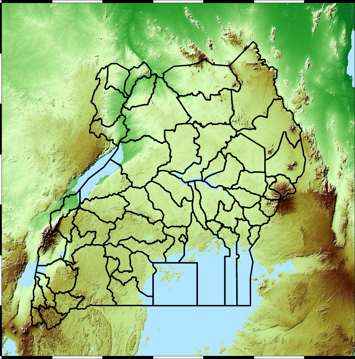
(Andrade-Pacheco et al., 2014; Mubangizi et al., 2014)

Kapchorwa District

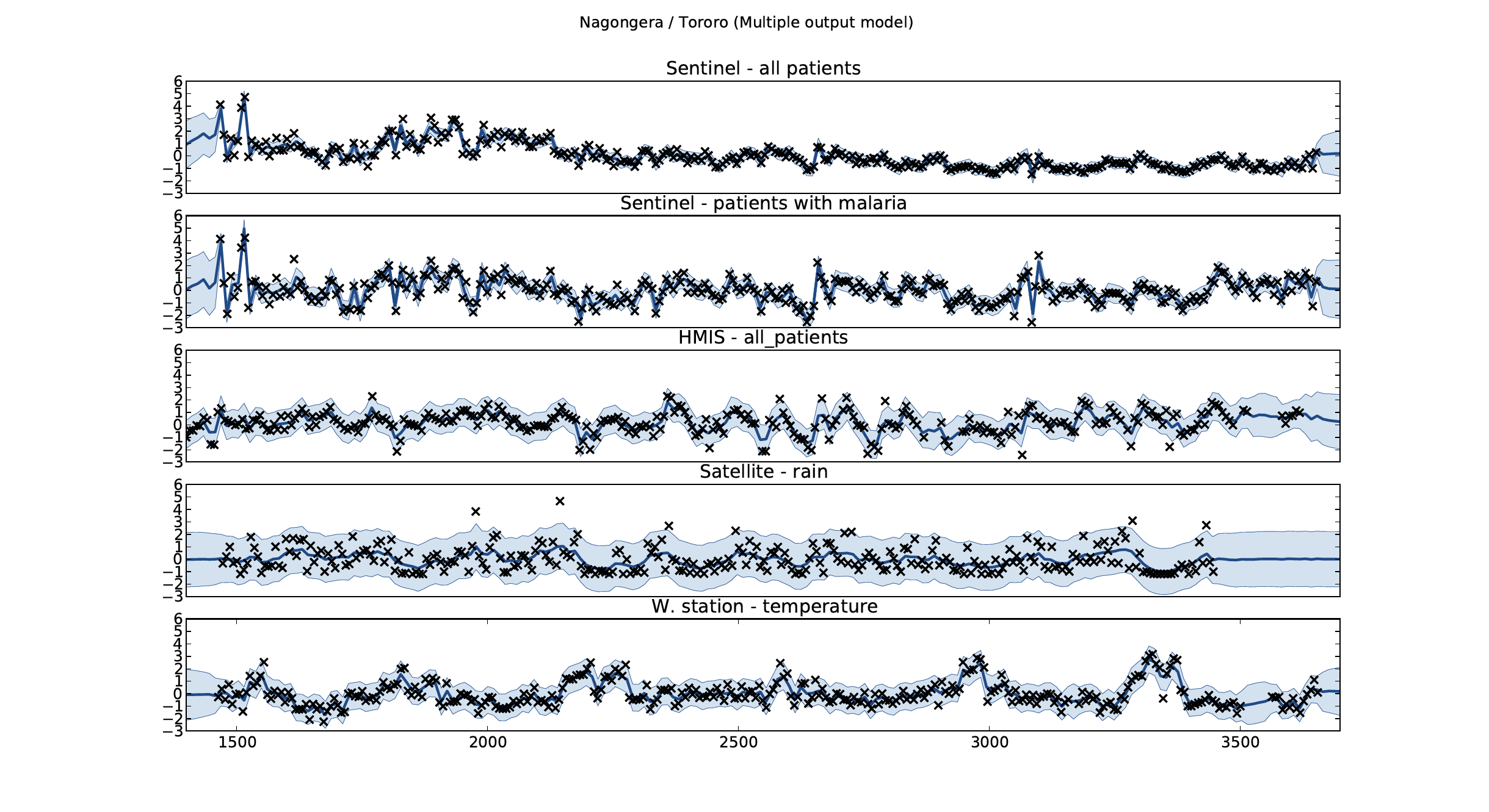
Tororo District

Malaria Prediction in Nagongera (Sentinel Site)

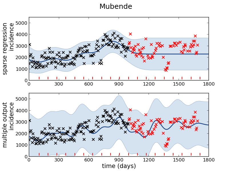
Mubende District

Malaria Prediction in Uganda

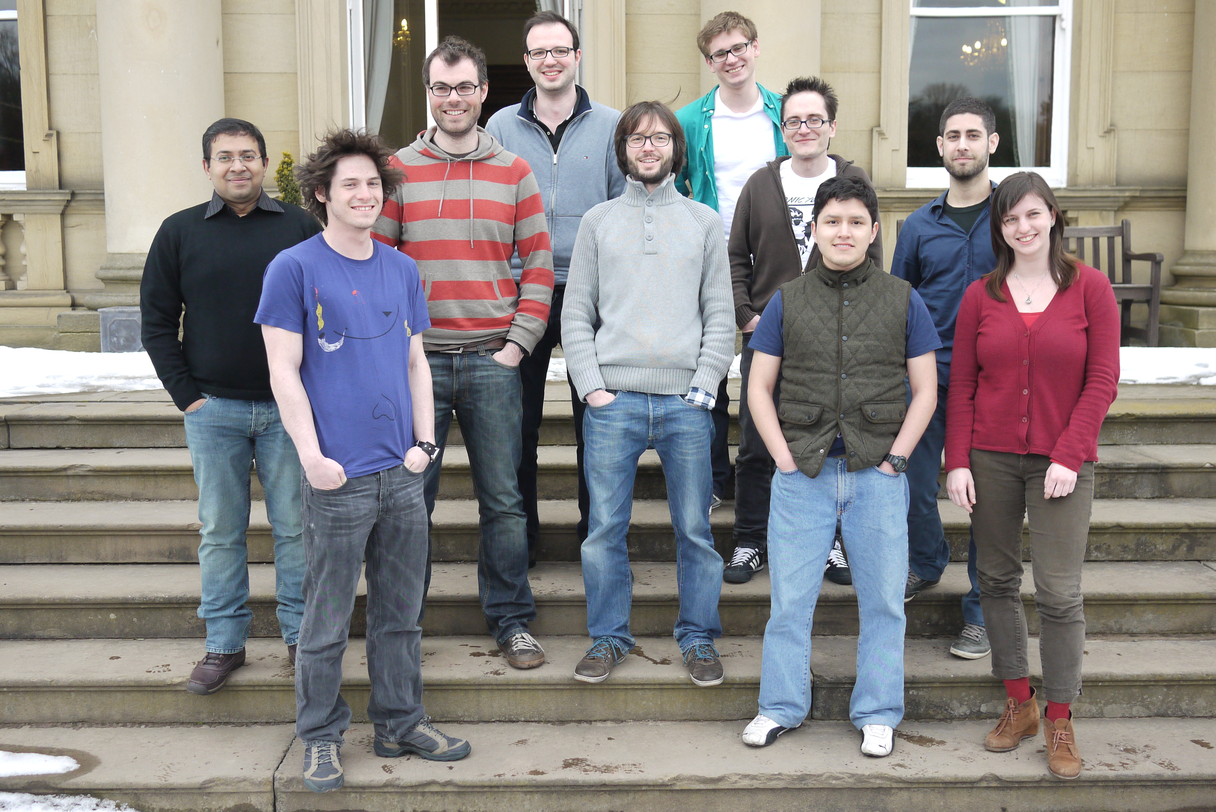
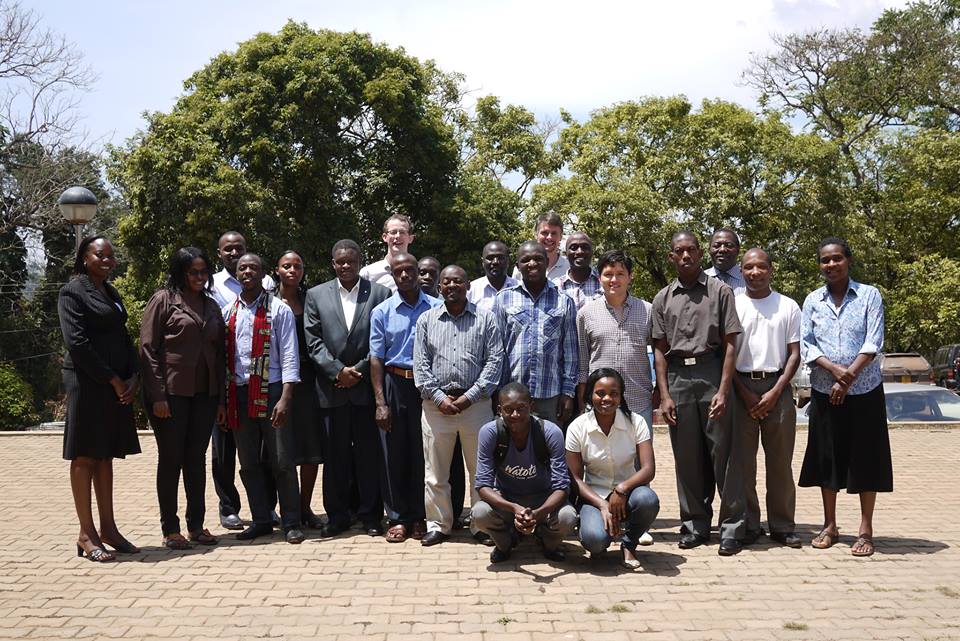
GP School at Makerere

Early Warning Systems

Kabarole District

Early Warning Systems

Additive Covariance

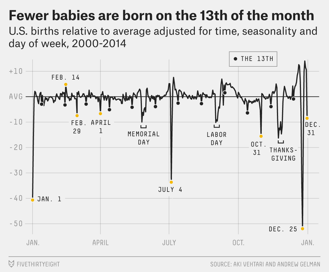
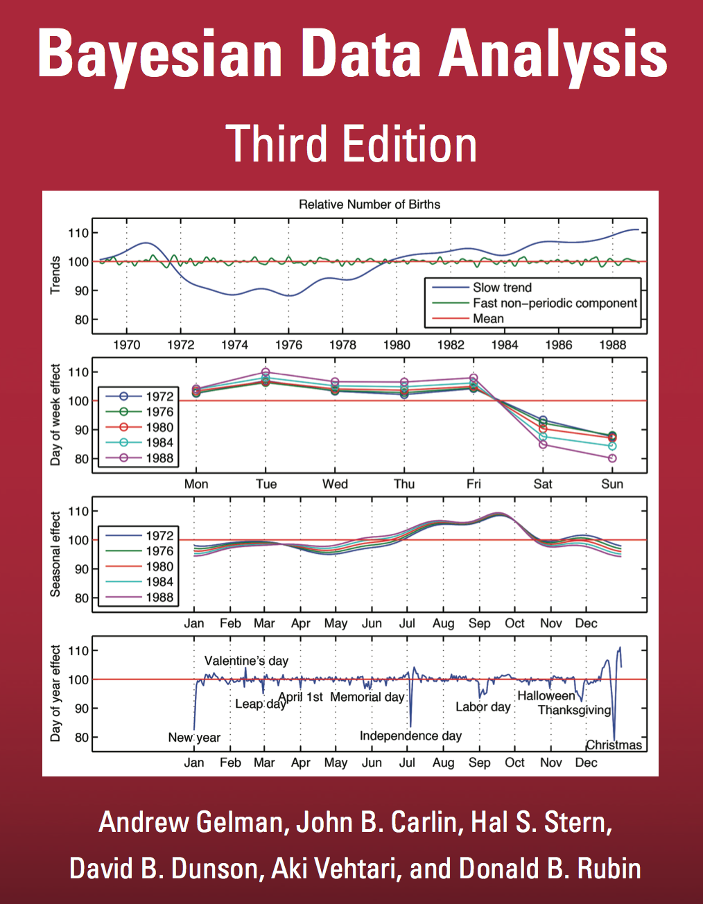
Gelman Book

Gelman et al. (2013)

Basis Function Covariance

Brownian Covariance

MLP Covariance

GPSS: Gaussian Process Summer School

GPy: A Gaussian Process Framework in Python

GPy: A Gaussian Process Framework in Python

• BSD Licensed software base.
• Wide availability of libraries, ‘modern’ scripting language.
• Allows us to set projects to undergraduates in Comp Sci that use GPs.
• Available through GitHub https://github.com/SheffieldML/GPy
• Reproducible Research with Jupyter Notebook.

Features

• Probabilistic-style programming (specify the model, not the algorithm).
• Non-Gaussian likelihoods.
• Multivariate outputs.
• Dimensionality reduction.
• Approximations for large data sets.

Other Software

• GPflow
• GPyTorch

MXFusion: Modular Probabilistic Programming on MXNet

MxFusion

Work by Eric Meissner and Zhenwen Dai. Probabilistic programming. Available on Github

Acknowledgments

Stefanos Eleftheriadis, John Bronskill, Hugh Salimbeni, Rich Turner, Zhenwen Dai, Javier Gonzalez, Andreas Damianou, Mark Pullin, Michael Smith, James Hensman, John Quinn, Martin Mubangizi.

Thanks!

• twitter: @lawrennd
• podcast: The Talking Machines

• newspaper: Guardian Profile Page

• Blog post on What is Machine Learning?

References

Andrade-Pacheco, R., Mubangizi, M., Quinn, J., Lawrence, N.D., 2014. Consistent mapping of government malaria records across a changing territory delimitation. Malaria Journal 13. https://doi.org/10.1186/1475-2875-13-S1-P5
Cho, Y., Saul, L.K., 2009. Kernel methods for deep learning, in: Bengio, Y., Schuurmans, D., Lafferty, J.D., Williams, C.K.I., Culotta, A. (Eds.), Advances in Neural Information Processing Systems 22. Curran Associates, Inc., pp. 342–350.
Della Gatta, G., Bansal, M., Ambesi-Impiombato, A., Antonini, D., Missero, C., Bernardo, D. di, 2008. Direct targets of the trp63 transcription factor revealed by a combination of gene expression profiling and reverse engineering. Genome Research 18, 939–948. https://doi.org/10.1101/gr.073601.107
Gelman, A., Carlin, J.B., Stern, H.S., Rubin, D.B., 2013. Bayesian data analysis, 3rd ed. Chapman; Hall.
Ioffe, S., Szegedy, C., 2015. Batch normalization: Accelerating deep network training by reducing internal covariate shift, in: Bach, F., Blei, D. (Eds.), Proceedings of the 32nd International Conference on Machine Learning, Proceedings of Machine Learning Research. PMLR, Lille, France, pp. 448–456.
Kalaitzis, A.A., Lawrence, N.D., 2011. A simple approach to ranking differentially expressed gene expression time courses through Gaussian process regression. BMC Bioinformatics 12. https://doi.org/10.1186/1471-2105-12-180
MacKay, D.J.C., 1992. Bayesian methods for adaptive models (PhD thesis). California Institute of Technology.
McCulloch, W.S., Pitts, W., 1943. A logical calculus of the ideas immanent in nervous activity. Bulletin of Mathematical Biophysics 5, 115–133.
Mubangizi, M., Andrade-Pacheco, R., Smith, M.T., Quinn, J., Lawrence, N.D., 2014. Malaria surveillance with multiple data sources using Gaussian process models, in: 1st International Conference on the Use of Mobile Ict in Africa.
Neal, R.M., 1994. Bayesian learning for neural networks (PhD thesis). Dept. of Computer Science, University of Toronto.
Rasmussen, C.E., Williams, C.K.I., 2006. Gaussian processes for machine learning. mit, Cambridge, MA.
Steele, S., Bilchik, A., Eberhardt, J., Kalina, P., Nissan, A., Johnson, E., Avital, I., Stojadinovic, A., 2012. Using machine-learned Bayesian belief networks to predict perioperative risk of clostridium difficile infection following colon surgery. Interact J Med Res 1, e6. https://doi.org/10.2196/ijmr.2131
Tipping, M.E., Bishop, C.M., 1999. Probabilistic principal component analysis. Journal of the Royal Statistical Society, B 6, 611–622. https://doi.org/doi:10.1111/1467-9868.00196