Machine Learning Systems Design
The Three Ds of Machine Learning
Data Science Africa, Addis Ababa

\[\text{data} + \text{model} \xrightarrow{\text{compute}} \text{prediction}\]
From Model to Decision

|
\[\text{data} + \text{model} \xrightarrow{\text{compute}} \text{prediction}\] |
Artificial Intelligence and Data Science
- AI aims to equip computers with human capabilities
- Image understanding
- Computer vision
- Speech recognition
- Natural language understanding
- Machine translation
Supervised Learning for AI
- Dominant approach today:
- Generate large labelled data set from humans.
- Use supervised learning to emulate that data.
- E.g. ImageNet Russakovsky et al. (2015)
- Significant advances due to deep learning
- E.g. Alexa, Amazon Go
Data Science
- Arises from happenstance data.
- Differs from statistics in that the question comes after data collection.
Amazon: Bits and Atoms
Supply Chain

Cromford

Deep Freeze

Deep Freeze
Machine Learning in Supply Chain
- Supply chain: Large Automated Decision Making Network
- Major Challenge:
- We have a mechanistic understanding of supply chain.
- Machine learning is a data driven technology.
Motto
Solve Supply Chain, then solve everything else.
The Three Ds of Machine Learning Systems Design
- Three primary challenges of Machine Learning Systems Design.
- Decomposition
- Data
- Deployment
Decomposition
- ML is not Magical Pixie Dust.
- It cannot be sprinkled thoughtlessly.
- We cannot simply automate all decisions through data
Decomposition
We are constrained by:
- Our data.
- The models.
Decomposition of Task
- Careful thought needs to be put into sub-processes of task.
- Any repetitive task is a candidate for automation.
Pigeonholing
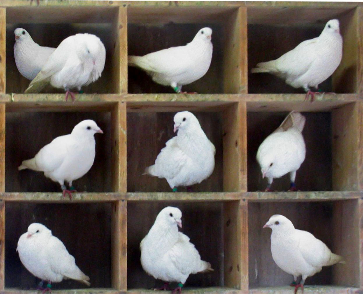
Pigeonholing
- Can we decompose decision we need to repetitive sub-tasks where inputs and outputs are well defined?
- Are those repetitive sub-tasks well represent by a mathematical mapping?
A Trap
- Over emphasis on the type of model we’re deploying.
- Under emphasis on the appropriateness of the task decomposition.
Chicken and Egg

Co-evolution
- Absolute decomposition is impossible.
- If we deploy a weak component in one place, downstream system will compensate.
- Systems co-evolve … there is no simple solution
- Trade off between performance and decomposability.
- Need to monitor deployment
Data
- Hard to overstate its importance.
- Half the equation of \(\text{data} + \text{model}\).
- Often utterly neglected.
Data Neglect
- Arises for two reasons.
- Data cleaning is perceived as tedious.
- Data cleaning is complex.
Data Cleaning
- Seems difficult to formulate into readily teachable princples.
- Heavily neglected in data science, statistics and ML courses.
- In practice most scientists spend around 80% of time data cleaning.
The Software Crisis
The major cause of the software crisis is that the machines have become several orders of magnitude more powerful! To put it quite bluntly: as long as there were no machines, programming was no problem at all; when we had a few weak computers, programming became a mild problem, and now we have gigantic computers, programming has become an equally gigantic problem.
Edsger Dijkstra (1930-2002), The Humble Programmer
The Data Crisis
The major cause of the data crisis is that machines have become more interconnected than ever before. Data access is therefore cheap, but data quality is often poor. What we need is cheap high-quality data. That implies that we develop processes for improving and verifying data quality that are efficient.
There would seem to be two ways for improving efficiency. Firstly, we should not duplicate work. Secondly, where possible we should automate work.
Me
Data Readiness Levels
https://arxiv.org/pdf/1705.02245.pdf Data Readiness Levels (Lawrence, 2017)
Three Grades of Data Readiness
- Grade C - accessibility
- Transition: data becomes electronically available
- Grade B - validity
- Transition: pose a question to the data.
- Grade A - usability
Data Science as Debugging
- Analogies: For Software Engineers describe data science as debugging.
80/20 in Data Science
- Anecdotally for a given challenge
- 80% of time is spent on data wrangling.
- 20% of time spent on modelling.
- Many companies employ ML Engineers focussing on models not data.

Deployment
Premise
Our machine learning is based on a software systems view that is 20 years out of date.
Continuous Deployment
- Deployment of modeling code.
- Data dependent models in production need continuous monitoring.
- Continous monitoring implies statistical tests rather than classic software tests.
Continuous Monitoring
- Continuous deployment:
- We’ve changed the code, we should test the effect.
- Continuous Monitoring:
- The world around us is changing, we should monitor the effect.
- Update our notions of testing: progression testing
Data Oriented Architectures
- Convert data to a first-class citizen.
- View system as operations on data streams.
- Expose data operations in a programmatic way.
Data Orientated Architectures
- Historically we’ve been software first
- A necessary but not sufficient condition for data first
- Move from
- service orientated architectures
- data orientated architectures
Streaming System
- Move from pull updates to push updates.
- Operate on rows rather than columns.
- Lead to stateless logic: persistence handled by system.
- Example Apache Kafka + Apache Flink
Streaming Architectures
- AWS Kinesis, Apache Kafka
- Not just about streaming
- Nodes in the architecture are stateless
- They persist through storing state on streams
- This brings the data inside out
Apache Flink
- Streams and transformations
- a stream is a (potentially never-ending) flow of data records
- a transformation: streams as input, produces transformed streams as output
Join
stream.join(otherStream)
    .where(<KeySelector>)
    .equalTo(<KeySelector>)
    .window(<WindowAssigner>)
    .apply(<JoinFunction>)
Milan
- Data Oriented Programming Language and runtime.
- DSL Embedded in Scala converts to an intermediate langugage.
- Intermediate language for compilation on different platforms (currently Flink)
Trading System
- High frequency share trading.
- Stream of prices with millisecond updates.
- Trades required on millisecond time line
Real Price
Future Price
Hypothetical Streams
- Real stream — share prices
- derived hypothetical stream — share prices in future.
- Hypothetical constrained by
- input constraints.
- decision functional
- computational requirements (latency)
Hypothetical Advantage
- Modelling is now required.
- But modelling is declared in the ecosystem.
- If it’s manual, warnings can be used
- calibration, fairness, dataset shift
- Opens door to Auto AI.
SafeBoda

SafeBoda
With road accidents set to match HIV/AIDS as the highest cause of death in low/middle income countries by 2030, SafeBoda’s aim is to modernise informal transportation and ensure safe access to mobility.
Ride Allocation Prediction
Ride Sharing: Service Oriented
Ride Sharing: Data Oriented
Ride Sharing: Hypothetical
Information Dynamics
- Potential for information feedback loops.
- Hypothetical streams are instantiated.
- Nature hypothesis (e.g. price prediction) can effect reality.
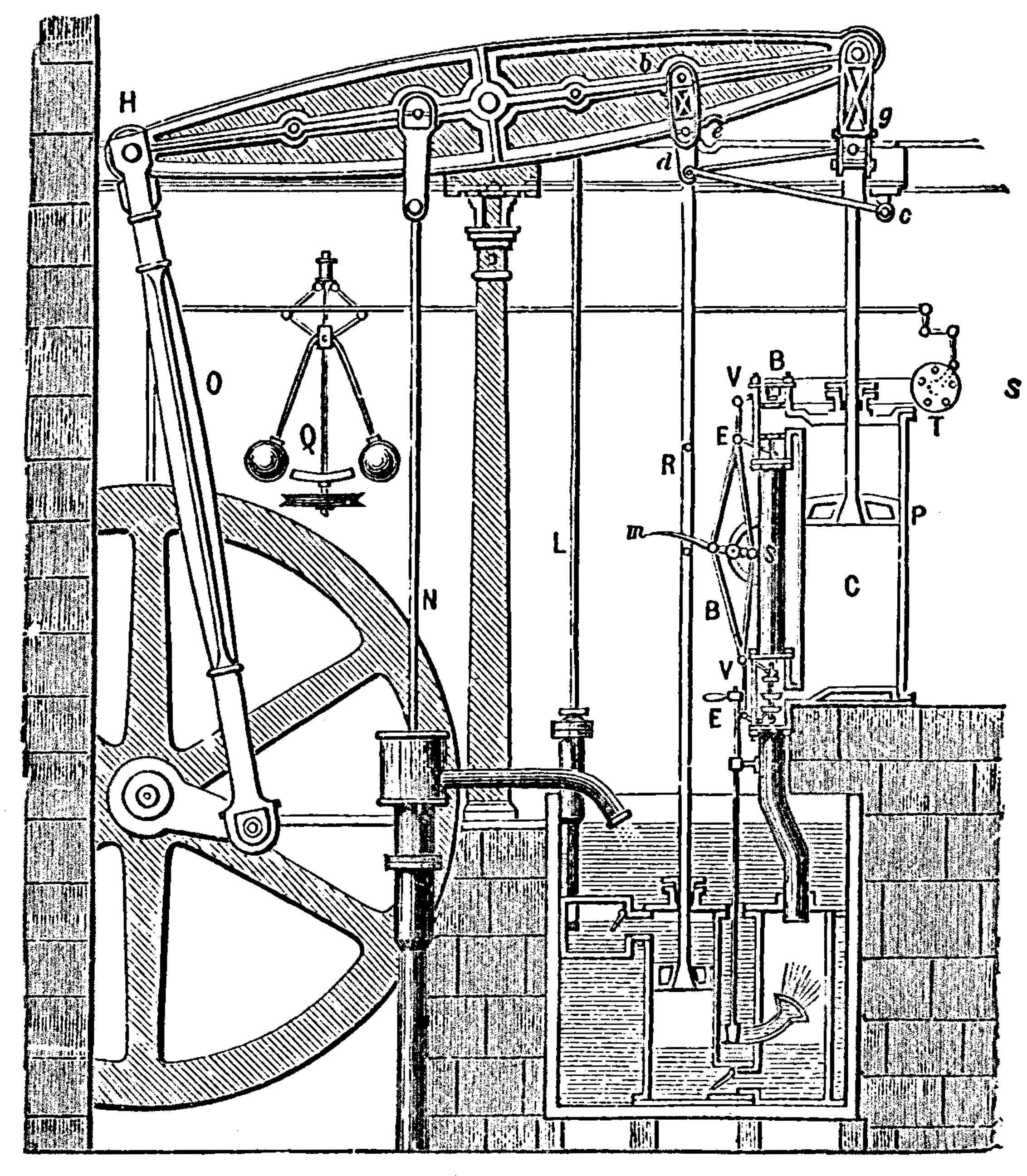
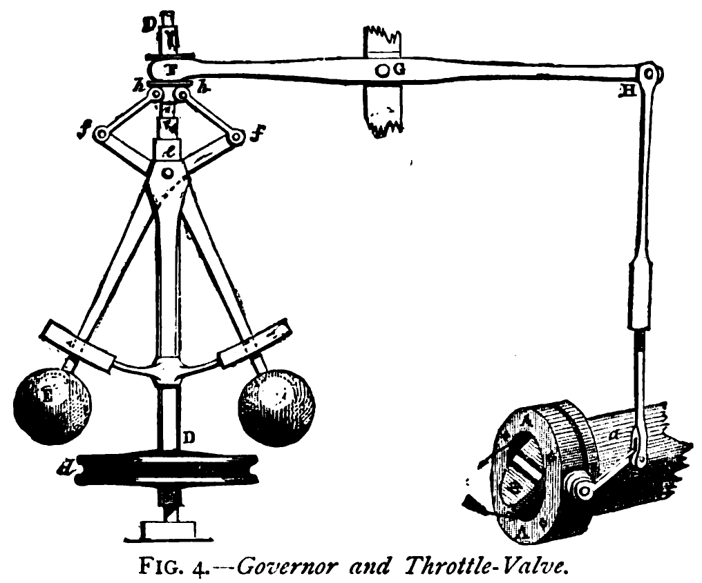
- Leads to information dynamics, similar to dynamics of governors.
- See e.g. Closed Loop Data Science at Glasgow.
Conclusion
- Challenges in decomposition, data and model deployment for ML.
- Data oriented architectures and data first thinking are the solution.
- Data oriented programming creates systems that are ready to deploy.
- Opens the door to AutoAI and information dynamics analysis.
Thanks!
- twitter: @lawrennd
- podcast: The Talking Machines
- newspaper: Guardian Profile Page
Blog post on The 3Ds of Machine Learning Systems Design
Blog post on Data Readiness Levels
Blog post on Data Science as Debugging
References
Lawrence, N.D., 2017. Data readiness levels. arXiv.
Russakovsky, O., Deng, J., Su, H., Krause, J., Satheesh, S., Ma, S., Huang, Z., Karpathy, A., Khosla, A., Bernstein, M., Berg, A.C., Fei-Fei, L., 2015. ImageNet Large Scale Visual Recognition Challenge. International Journal of Computer Vision (IJCV) 115, 211–252. https://doi.org/10.1007/s11263-015-0816-y