Interpretable End-to-End Learning

Bits and Atoms

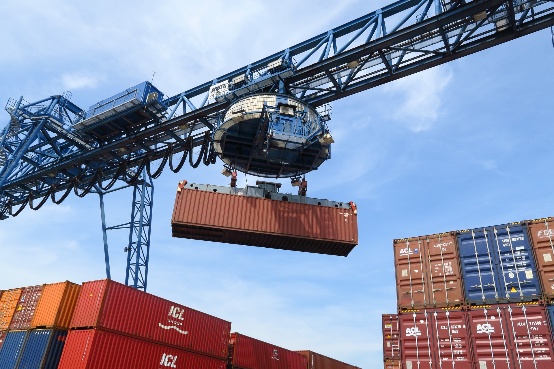
Supply Chain

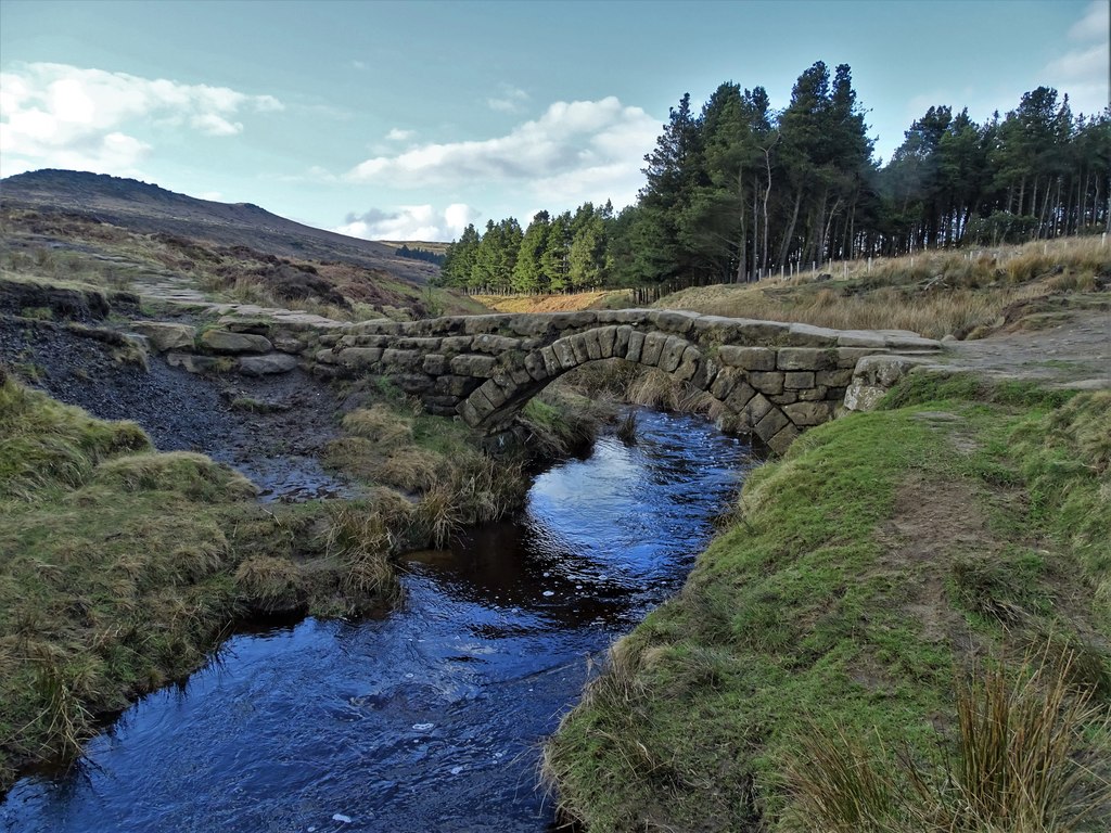
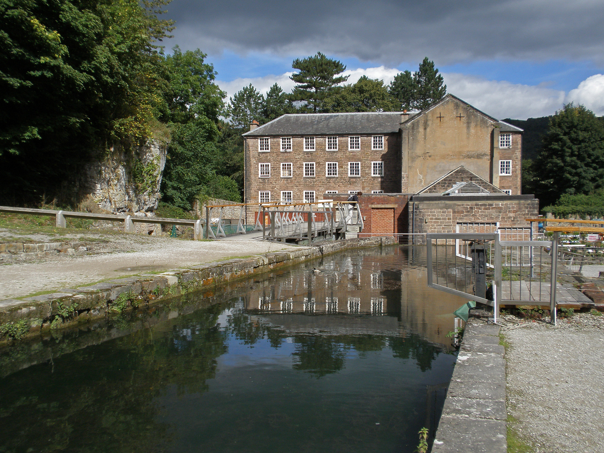
Cromford

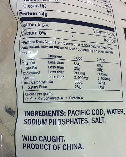
Deep Freeze

Machine Learning in Supply Chain

Supply chain: Large Automated Decision Making Network
Major Challenge:
- We have a mechanistic understanding of supply chain.
- Machine learning is a data driven technology.

Motto

Solve Supply Chain, then solve everything else.

From Model to Decision

\[\text{data} + \text{model} \xrightarrow{\text{compute}} \text{prediction}\]

Experiment, Analyze, Design

Our Vision

We don’t know what science we’ll want to do in 5 years time, but we won’t want slower experiments, we won’t want more expensive experiments and we won’t want a narrower selection of experiments.

What do we want?

Faster, cheaper and more diverse experiments.
Better ecosystems for experimentation.
Data oriented architectures.

Data Oriented Architectures

Convert data to a first-class citizen.
View system as operations on data streams.
Expose data operations in a programmatic way.

Data Orientated Architectures

Historically we’ve been software first
- A necessary but not sufficient condition for data first
Move from
1. service orientated architectures
2. data orientated architectures

Streaming System

Move from pull updates to push updates.
Operate on rows rather than columns.
Lead to stateless logic: persistence handled by system.
Example Apache Kafka + Apache Flink

Streaming Architectures

AWS Kinesis, Apache Kafka
Not just about streaming
- Nodes in the architecture are stateless
- They persist through storing state on streams
This brings the data inside out

Apache Flink

Streams and transformations
a stream is a (potentially never-ending) flow of data records
a transformation: streams as input, produces transformed streams as output

Join

stream.join(otherStream)
    .where(<KeySelector>)
    .equalTo(<KeySelector>)
    .window(<WindowAssigner>)
    .apply(<JoinFunction>)

Milan

Data Oriented Programming Language and runtime.
DSL Embedded in Scala converts to an intermediate langugage.
Intermediate language for compilation on different platforms (currently Flink)

https://github.com/amzn/milan

Trading System

High frequency share trading.
Stream of prices with millisecond updates.
Trades required on millisecond time line

Real Price

Future Price

Hypothetical Streams

Real stream — share prices
- derived hypothetical stream — share prices in future.
Hypothetical constrained by
- input constraints.
- decision functional
- computational requirements (latency)

Hypothetical Advantage

Modelling is now required.
But modelling is declared in the ecosystem.
If it’s manual, warnings can be used
- calibration, fairness, dataset shift
Opens door to Auto AI.

SafeBoda

With road accidents set to match HIV/AIDS as the highest cause of death in low/middle income countries by 2030, SafeBoda’s aim is to modernise informal transportation and ensure safe access to mobility.

Ride Allocation Prediction

Ride Sharing: Service Oriented

Ride Sharing: Data Oriented

Ride Sharing: Hypothetical

Information Dynamics

Potential for information feedback loops.
Hypothetical streams are instantiated.
Nature hypothesis (e.g. price prediction) can effect reality.
Leads to information dynamics, similar to dynamics of governors.
See e.g. Closed Loop Data Science at Glasgow.

Autonomous Vehicles

Emulation

Deep Emulation

Bayesian System Optimization

Aim: maintain interpretable components.
Monitor downstream/upstream effects through emulation.
Optimize individual components considering upstream and downstream.

Auto AI

Auto ML is great but not sufficient
Interacting components in an ML system
Identify problems, and automatically deploy solutions

Technology: Deep Emulation

DeepFace

Outline of the DeepFace architecture. A front-end of a single convolution-pooling-convolution filtering on the rectified input, followed by three locally-connected layers and two fully-connected layers. Color illustrates feature maps produced at each layer. The net includes more than 120 million parameters, where more than 95% come from the local and fully connected.

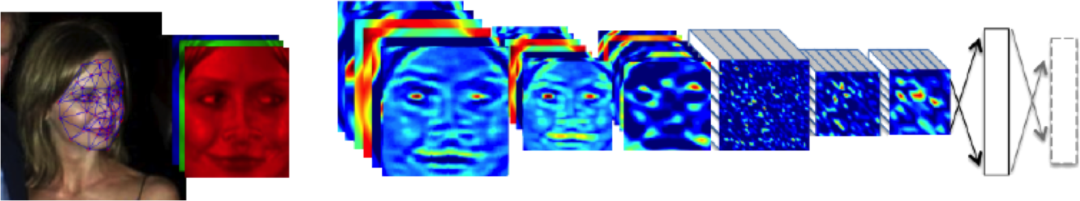
Source: DeepFace (Taigman et al., 2014)

Deep Neural Network

Mathematically

\[ \begin{align} \hiddenVector_{1} &= \basisFunction\left(\mappingMatrix_1 \inputVector\right)\\ \hiddenVector_{2} &= \basisFunction\left(\mappingMatrix_2\hiddenVector_{1}\right)\\ \hiddenVector_{3} &= \basisFunction\left(\mappingMatrix_3 \hiddenVector_{2}\right)\\ \dataVector &= \mappingVector_4 ^\top\hiddenVector_{3} \end{align} \]

Overfitting

Potential problem: if number of nodes in two adjacent layers is big, corresponding \(\mappingMatrix\) is also very big and there is the potential to overfit.
Proposed solution: “dropout”.
Alternative solution: parameterize \(\mappingMatrix\) with its SVD. \[ \mappingMatrix = \eigenvectorMatrix\eigenvalueMatrix\eigenvectwoMatrix^\top \] or \[ \mappingMatrix = \eigenvectorMatrix\eigenvectwoMatrix^\top \] where if \(\mappingMatrix \in \Re^{k_1\times k_2}\) then \(\eigenvectorMatrix\in \Re^{k_1\times q}\) and \(\eigenvectwoMatrix \in \Re^{k_2\times q}\), i.e. we have a low rank matrix factorization for the weights.

Low Rank Approximation

Bottleneck Layers in Deep Neural Networks

Deep Neural Network

Mathematically

The network can now be written mathematically as \[ \begin{align} \latentVector_{1} &= \eigenvectwoMatrix^\top_1 \inputVector\\ \hiddenVector_{1} &= \basisFunction\left(\eigenvectorMatrix_1 \latentVector_{1}\right)\\ \latentVector_{2} &= \eigenvectwoMatrix^\top_2 \hiddenVector_{1}\\ \hiddenVector_{2} &= \basisFunction\left(\eigenvectorMatrix_2 \latentVector_{2}\right)\\ \latentVector_{3} &= \eigenvectwoMatrix^\top_3 \hiddenVector_{2}\\ \hiddenVector_{3} &= \basisFunction\left(\eigenvectorMatrix_3 \latentVector_{3}\right)\\ \dataVector &= \mappingVector_4^\top\hiddenVector_{3}. \end{align} \]

A Cascade of Neural Networks

\[ \begin{align} \latentVector_{1} &= \eigenvectwoMatrix^\top_1 \inputVector\\ \latentVector_{2} &= \eigenvectwoMatrix^\top_2 \basisFunction\left(\eigenvectorMatrix_1 \latentVector_{1}\right)\\ \latentVector_{3} &= \eigenvectwoMatrix^\top_3 \basisFunction\left(\eigenvectorMatrix_2 \latentVector_{2}\right)\\ \dataVector &= \mappingVector_4 ^\top \latentVector_{3} \end{align} \]

Cascade of Gaussian Processes

Replace each neural network with a Gaussian process \[ \begin{align} \latentVector_{1} &= \mappingFunctionVector_1\left(\inputVector\right)\\ \latentVector_{2} &= \mappingFunctionVector_2\left(\latentVector_{1}\right)\\ \latentVector_{3} &= \mappingFunctionVector_3\left(\latentVector_{2}\right)\\ \dataVector &= \mappingFunctionVector_4\left(\latentVector_{3}\right) \end{align} \]
Equivalent to prior over parameters, take width of each layer to infinity.

Stochastic Process Composition

\[\dataVector = \mappingFunctionVector_4\left(\mappingFunctionVector_3\left(\mappingFunctionVector_2\left(\mappingFunctionVector_1\left(\inputVector\right)\right)\right)\right)\]

Motorcycle Helmet Data

Motorcycle Helmet Data GP

Motorcycle Helmet Data Deep GP

Motorcycle Helmet Data Latent 1

Motorcycle Helmet Data Latent 2

Motorcycle Helmet Pinball Plot

Graphical Models

Represent joint distribution through conditional dependencies.
E.g. Markov chain

\[p(\dataVector) = p(\dataScalar_\numData | \dataScalar_{\numData-1}) p(\dataScalar_{\numData-1}|\dataScalar_{\numData-2}) \dots p(\dataScalar_{2} | \dataScalar_{1})\]

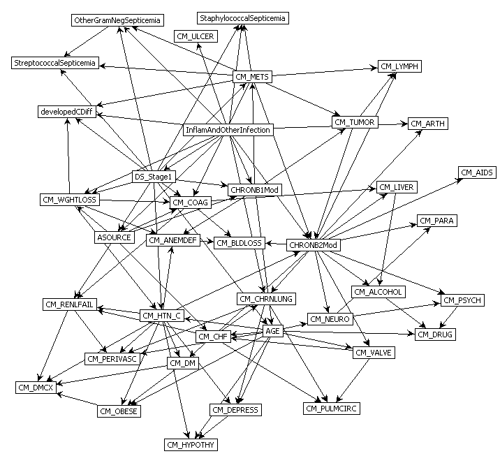
Predict Perioperative Risk of Clostridium Difficile Infection Following Colon Surgery (Steele et al., 2012)

Conclusion

Challenges in decomposition, data and model deployment for ML.
Data oriented architectures and data first thinking are the solution.
Data oriented programming creates systems that are ready to deploy.
Opens the door to AutoAI and information dynamics analysis.

Related Papers

Deep Gaussian Processes Damianou and Lawrence (2013)
Latent Force Models Álvarez et al. (2013)
Gaussian Process Latent Force Models for Learning and Stochastic Control of Physical Systems Särkkä et al. (2018)
The Emergence of Organizing Structure in Conceptual Representation Lake et al. (2018)

Other’s Work

How Deep Are Deep Gaussian Processes? Dunlop et al. (n.d.)
Doubly Stochastic Variational Inference for Deep Gaussian Processes Salimbeni and Deisenroth (2017)
Deep Multi-task Gaussian Processes for Survival Analysis with Competing Risks Alaa and van der Schaar (2017)
Counterfactual Gaussian Processes for Reliable Decision-making and What-if Reasoning Schulam and Saria (2017)

Conclusions and Directions

Mechanistic modelling
Automated Abstraction
Deep emulation
Bayesian Systems Optimization
Auto AI

Thanks!

References

Alaa, A.M., van der Schaar, M., 2017. Deep multi-task Gaussian processes for survival analysis with competing risks, in: Guyon, I., Luxburg, U.V., Bengio, S., Wallach, H., Fergus, R., Vishwanathan, S., Garnett, R. (Eds.), Advances in Neural Information Processing Systems 30. Curran Associates, Inc., pp. 2326–2334.

Álvarez, M.A., Luengo, D., Lawrence, N.D., 2013. Linear latent force models using Gaussian processes. IEEE Transactions on Pattern Analysis and Machine Intelligence 35, 2693–2705. https://doi.org/10.1109/TPAMI.2013.86

Damianou, A., Lawrence, N.D., 2013. Deep Gaussian processes, in:. pp. 207–215.

Dunlop, M.M., Girolami, M.A., Stuart, A.M., Teckentrup, A.L., n.d. How deep are deep Gaussian processes? Journal of Machine Learning Research 19, 1–46.

Lake, B.M., Lawrence, N.D., Tenenbaum, J.B., 2018. The emergence of organizing structure in conceptual representation. Cognitive science 42 Suppl 3, 809–832. https://doi.org/10.1111/cogs.12580

Salimbeni, H., Deisenroth, M., 2017. Doubly stochastic variational inference for deep Gaussian processes, in: Guyon, I., Luxburg, U.V., Bengio, S., Wallach, H., Fergus, R., Vishwanathan, S., Garnett, R. (Eds.), Advances in Neural Information Processing Systems 30. Curran Associates, Inc., pp. 4591–4602.

Särkkä, S., Álvarez, M.A., Lawrence, N.D., 2018. Gaussian process latent force models for learning and stochastic control of physical systems. IEEE Transactions on Automatic Control. https://doi.org/10.1109/TAC.2018.2874749

Schulam, P., Saria, S., 2017. Counterfactual Gaussian processes for reliable decision-making and what-if reasoning, in: Guyon, I., Luxburg, U.V., Bengio, S., Wallach, H., Fergus, R., Vishwanathan, S., Garnett, R. (Eds.), Advances in Neural Information Processing Systems 30. Curran Associates, Inc., pp. 1696–1706.

Steele, S., Bilchik, A., Eberhardt, J., Kalina, P., Nissan, A., Johnson, E., Avital, I., Stojadinovic, A., 2012. Using machine-learned Bayesian belief networks to predict perioperative risk of clostridium difficile infection following colon surgery. Interact J Med Res 1, e6. https://doi.org/10.2196/ijmr.2131

Taigman, Y., Yang, M., Ranzato, M., Wolf, L., 2014. DeepFace: Closing the gap to human-level performance in face verification, in: Proceedings of the IEEE Computer Society Conference on Computer Vision and Pattern Recognition. https://doi.org/10.1109/CVPR.2014.220