\[\newcommand{\tk}[1]{} %\newcommand{\tk}[1]{\textbf{TK}: #1} \newcommand{\Amatrix}{\mathbf{A}} \newcommand{\KL}[2]{\text{KL}\left( #1\,\|\,#2 \right)} \newcommand{\Kaast}{\kernelMatrix_{\mathbf{ \ast}\mathbf{ \ast}}} \newcommand{\Kastu}{\kernelMatrix_{\mathbf{ \ast} \inducingVector}} \newcommand{\Kff}{\kernelMatrix_{\mappingFunctionVector \mappingFunctionVector}} \newcommand{\Kfu}{\kernelMatrix_{\mappingFunctionVector \inducingVector}} \newcommand{\Kuast}{\kernelMatrix_{\inducingVector \bf\ast}} \newcommand{\Kuf}{\kernelMatrix_{\inducingVector \mappingFunctionVector}} \newcommand{\Kuu}{\kernelMatrix_{\inducingVector \inducingVector}} \newcommand{\Kuui}{\Kuu^{-1}} \newcommand{\Qaast}{\mathbf{Q}_{\bf \ast \ast}} \newcommand{\Qastf}{\mathbf{Q}_{\ast \mappingFunction}} \newcommand{\Qfast}{\mathbf{Q}_{\mappingFunctionVector \bf \ast}} \newcommand{\Qff}{\mathbf{Q}_{\mappingFunctionVector \mappingFunctionVector}} \newcommand{\aMatrix}{\mathbf{A}} \newcommand{\aScalar}{a} \newcommand{\aVector}{\mathbf{a}} \newcommand{\acceleration}{a} \newcommand{\bMatrix}{\mathbf{B}} \newcommand{\bScalar}{b} \newcommand{\bVector}{\mathbf{b}} \newcommand{\basisFunc}{\phi} \newcommand{\basisFuncVector}{\boldsymbol{ \basisFunc}} \newcommand{\basisFunction}{\phi} \newcommand{\basisLocation}{\mu} \newcommand{\basisMatrix}{\boldsymbol{ \Phi}} \newcommand{\basisScalar}{\basisFunction} \newcommand{\basisVector}{\boldsymbol{ \basisFunction}} \newcommand{\activationFunction}{\phi} \newcommand{\activationMatrix}{\boldsymbol{ \Phi}} \newcommand{\activationScalar}{\basisFunction} \newcommand{\activationVector}{\boldsymbol{ \basisFunction}} \newcommand{\bigO}{\mathcal{O}} \newcommand{\binomProb}{\pi} \newcommand{\cMatrix}{\mathbf{C}} \newcommand{\cbasisMatrix}{\hat{\boldsymbol{ \Phi}}} \newcommand{\cdataMatrix}{\hat{\dataMatrix}} \newcommand{\cdataScalar}{\hat{\dataScalar}} \newcommand{\cdataVector}{\hat{\dataVector}} \newcommand{\centeredKernelMatrix}{\mathbf{ \MakeUppercase{\centeredKernelScalar}}} \newcommand{\centeredKernelScalar}{b} \newcommand{\centeredKernelVector}{\centeredKernelScalar} \newcommand{\centeringMatrix}{\mathbf{H}} \newcommand{\chiSquaredDist}[2]{\chi_{#1}^{2}\left(#2\right)} \newcommand{\chiSquaredSamp}[1]{\chi_{#1}^{2}} \newcommand{\conditionalCovariance}{\boldsymbol{ \Sigma}} \newcommand{\coregionalizationMatrix}{\mathbf{B}} \newcommand{\coregionalizationScalar}{b} \newcommand{\coregionalizationVector}{\mathbf{ \coregionalizationScalar}} \newcommand{\covDist}[2]{\text{cov}_{#2}\left(#1\right)} \newcommand{\covSamp}[1]{\text{cov}\left(#1\right)} \newcommand{\covarianceScalar}{c} \newcommand{\covarianceVector}{\mathbf{ \covarianceScalar}} \newcommand{\covarianceMatrix}{\mathbf{C}} \newcommand{\covarianceMatrixTwo}{\boldsymbol{ \Sigma}} \newcommand{\croupierScalar}{s} \newcommand{\croupierVector}{\mathbf{ \croupierScalar}} \newcommand{\croupierMatrix}{\mathbf{ \MakeUppercase{\croupierScalar}}} \newcommand{\dataDim}{p} \newcommand{\dataIndex}{i} \newcommand{\dataIndexTwo}{j} \newcommand{\dataMatrix}{\mathbf{Y}} \newcommand{\dataScalar}{y} \newcommand{\dataSet}{\mathcal{D}} \newcommand{\dataStd}{\sigma} \newcommand{\dataVector}{\mathbf{ \dataScalar}} \newcommand{\decayRate}{d} \newcommand{\degreeMatrix}{\mathbf{ \MakeUppercase{\degreeScalar}}} \newcommand{\degreeScalar}{d} \newcommand{\degreeVector}{\mathbf{ \degreeScalar}} % Already defined by latex %\newcommand{\det}[1]{\left|#1\right|} \newcommand{\diag}[1]{\text{diag}\left(#1\right)} \newcommand{\diagonalMatrix}{\mathbf{D}} \newcommand{\diff}[2]{\frac{\text{d}#1}{\text{d}#2}} \newcommand{\diffTwo}[2]{\frac{\text{d}^2#1}{\text{d}#2^2}} \newcommand{\displacement}{x} \newcommand{\displacementVector}{\textbf{\displacement}} \newcommand{\distanceMatrix}{\mathbf{ \MakeUppercase{\distanceScalar}}} \newcommand{\distanceScalar}{d} \newcommand{\distanceVector}{\mathbf{ \distanceScalar}} \newcommand{\eigenvaltwo}{\ell} \newcommand{\eigenvaltwoMatrix}{\mathbf{L}} \newcommand{\eigenvaltwoVector}{\mathbf{l}} \newcommand{\eigenvalue}{\lambda} \newcommand{\eigenvalueMatrix}{\boldsymbol{ \Lambda}} \newcommand{\eigenvalueVector}{\boldsymbol{ \lambda}} \newcommand{\eigenvector}{\mathbf{ \eigenvectorScalar}} \newcommand{\eigenvectorMatrix}{\mathbf{U}} \newcommand{\eigenvectorScalar}{u} \newcommand{\eigenvectwo}{\mathbf{v}} \newcommand{\eigenvectwoMatrix}{\mathbf{V}} \newcommand{\eigenvectwoScalar}{v} \newcommand{\entropy}[1]{\mathcal{H}\left(#1\right)} \newcommand{\errorFunction}{E} \newcommand{\expDist}[2]{\left<#1\right>_{#2}} \newcommand{\expSamp}[1]{\left<#1\right>} \newcommand{\expectation}[1]{\left\langle #1 \right\rangle } \newcommand{\expectationDist}[2]{\left\langle #1 \right\rangle _{#2}} \newcommand{\expectedDistanceMatrix}{\mathcal{D}} \newcommand{\eye}{\mathbf{I}} \newcommand{\fantasyDim}{r} \newcommand{\fantasyMatrix}{\mathbf{ \MakeUppercase{\fantasyScalar}}} \newcommand{\fantasyScalar}{z} \newcommand{\fantasyVector}{\mathbf{ \fantasyScalar}} \newcommand{\featureStd}{\varsigma} \newcommand{\gammaCdf}[3]{\mathcal{GAMMA CDF}\left(#1|#2,#3\right)} \newcommand{\gammaDist}[3]{\mathcal{G}\left(#1|#2,#3\right)} \newcommand{\gammaSamp}[2]{\mathcal{G}\left(#1,#2\right)} \newcommand{\gaussianDist}[3]{\mathcal{N}\left(#1|#2,#3\right)} \newcommand{\gaussianSamp}[2]{\mathcal{N}\left(#1,#2\right)} \newcommand{\given}{|} \newcommand{\half}{\frac{1}{2}} \newcommand{\heaviside}{H} \newcommand{\hiddenMatrix}{\mathbf{ \MakeUppercase{\hiddenScalar}}} \newcommand{\hiddenScalar}{h} \newcommand{\hiddenVector}{\mathbf{ \hiddenScalar}} \newcommand{\identityMatrix}{\eye} \newcommand{\inducingInputScalar}{z} \newcommand{\inducingInputVector}{\mathbf{ \inducingInputScalar}} \newcommand{\inducingInputMatrix}{\mathbf{Z}} \newcommand{\inducingScalar}{u} \newcommand{\inducingVector}{\mathbf{ \inducingScalar}} \newcommand{\inducingMatrix}{\mathbf{U}} \newcommand{\inlineDiff}[2]{\text{d}#1/\text{d}#2} \newcommand{\inputDim}{q} \newcommand{\inputMatrix}{\mathbf{X}} \newcommand{\inputScalar}{x} \newcommand{\inputSpace}{\mathcal{X}} \newcommand{\inputVals}{\inputVector} \newcommand{\inputVector}{\mathbf{ \inputScalar}} \newcommand{\iterNum}{k} \newcommand{\kernel}{\kernelScalar} \newcommand{\kernelMatrix}{\mathbf{K}} \newcommand{\kernelScalar}{k} \newcommand{\kernelVector}{\mathbf{ \kernelScalar}} \newcommand{\kff}{\kernelScalar_{\mappingFunction \mappingFunction}} \newcommand{\kfu}{\kernelVector_{\mappingFunction \inducingScalar}} \newcommand{\kuf}{\kernelVector_{\inducingScalar \mappingFunction}} \newcommand{\kuu}{\kernelVector_{\inducingScalar \inducingScalar}} \newcommand{\lagrangeMultiplier}{\lambda} \newcommand{\lagrangeMultiplierMatrix}{\boldsymbol{ \Lambda}} \newcommand{\lagrangian}{L} \newcommand{\laplacianFactor}{\mathbf{ \MakeUppercase{\laplacianFactorScalar}}} \newcommand{\laplacianFactorScalar}{m} \newcommand{\laplacianFactorVector}{\mathbf{ \laplacianFactorScalar}} \newcommand{\laplacianMatrix}{\mathbf{L}} \newcommand{\laplacianScalar}{\ell} \newcommand{\laplacianVector}{\mathbf{ \ell}} \newcommand{\latentDim}{q} \newcommand{\latentDistanceMatrix}{\boldsymbol{ \Delta}} \newcommand{\latentDistanceScalar}{\delta} \newcommand{\latentDistanceVector}{\boldsymbol{ \delta}} \newcommand{\latentForce}{f} \newcommand{\latentFunction}{u} \newcommand{\latentFunctionVector}{\mathbf{ \latentFunction}} \newcommand{\latentFunctionMatrix}{\mathbf{ \MakeUppercase{\latentFunction}}} \newcommand{\latentIndex}{j} \newcommand{\latentScalar}{z} \newcommand{\latentVector}{\mathbf{ \latentScalar}} \newcommand{\latentMatrix}{\mathbf{Z}} \newcommand{\learnRate}{\eta} \newcommand{\lengthScale}{\ell} \newcommand{\rbfWidth}{\ell} \newcommand{\likelihoodBound}{\mathcal{L}} \newcommand{\likelihoodFunction}{L} \newcommand{\locationScalar}{\mu} \newcommand{\locationVector}{\boldsymbol{ \locationScalar}} \newcommand{\locationMatrix}{\mathbf{M}} \newcommand{\variance}[1]{\text{var}\left( #1 \right)} \newcommand{\mappingFunction}{f} \newcommand{\mappingFunctionMatrix}{\mathbf{F}} \newcommand{\mappingFunctionTwo}{g} \newcommand{\mappingFunctionTwoMatrix}{\mathbf{G}} \newcommand{\mappingFunctionTwoVector}{\mathbf{ \mappingFunctionTwo}} \newcommand{\mappingFunctionVector}{\mathbf{ \mappingFunction}} \newcommand{\scaleScalar}{s} \newcommand{\mappingScalar}{w} \newcommand{\mappingVector}{\mathbf{ \mappingScalar}} \newcommand{\mappingMatrix}{\mathbf{W}} \newcommand{\mappingScalarTwo}{v} \newcommand{\mappingVectorTwo}{\mathbf{ \mappingScalarTwo}} \newcommand{\mappingMatrixTwo}{\mathbf{V}} \newcommand{\maxIters}{K} \newcommand{\meanMatrix}{\mathbf{M}} \newcommand{\meanScalar}{\mu} \newcommand{\meanTwoMatrix}{\mathbf{M}} \newcommand{\meanTwoScalar}{m} \newcommand{\meanTwoVector}{\mathbf{ \meanTwoScalar}} \newcommand{\meanVector}{\boldsymbol{ \meanScalar}} \newcommand{\mrnaConcentration}{m} \newcommand{\naturalFrequency}{\omega} \newcommand{\neighborhood}[1]{\mathcal{N}\left( #1 \right)} \newcommand{\neilurl}{http://inverseprobability.com/} \newcommand{\noiseMatrix}{\boldsymbol{ E}} \newcommand{\noiseScalar}{\epsilon} \newcommand{\noiseVector}{\boldsymbol{ \epsilon}} \newcommand{\norm}[1]{\left\Vert #1 \right\Vert} \newcommand{\normalizedLaplacianMatrix}{\hat{\mathbf{L}}} \newcommand{\normalizedLaplacianScalar}{\hat{\ell}} \newcommand{\normalizedLaplacianVector}{\hat{\mathbf{ \ell}}} \newcommand{\numActive}{m} \newcommand{\numBasisFunc}{m} \newcommand{\numComponents}{m} \newcommand{\numComps}{K} \newcommand{\numData}{n} \newcommand{\numFeatures}{K} \newcommand{\numHidden}{h} \newcommand{\numInducing}{m} \newcommand{\numLayers}{\ell} \newcommand{\numNeighbors}{K} \newcommand{\numSequences}{s} \newcommand{\numSuccess}{s} \newcommand{\numTasks}{m} \newcommand{\numTime}{T} \newcommand{\numTrials}{S} \newcommand{\outputIndex}{j} \newcommand{\paramVector}{\boldsymbol{ \theta}} \newcommand{\parameterMatrix}{\boldsymbol{ \Theta}} \newcommand{\parameterScalar}{\theta} \newcommand{\parameterVector}{\boldsymbol{ \parameterScalar}} \newcommand{\partDiff}[2]{\frac{\partial#1}{\partial#2}} \newcommand{\precisionScalar}{j} \newcommand{\precisionVector}{\mathbf{ \precisionScalar}} \newcommand{\precisionMatrix}{\mathbf{J}} \newcommand{\pseudotargetScalar}{\widetilde{y}} \newcommand{\pseudotargetVector}{\mathbf{ \pseudotargetScalar}} \newcommand{\pseudotargetMatrix}{\mathbf{ \widetilde{Y}}} \newcommand{\rank}[1]{\text{rank}\left(#1\right)} \newcommand{\rayleighDist}[2]{\mathcal{R}\left(#1|#2\right)} \newcommand{\rayleighSamp}[1]{\mathcal{R}\left(#1\right)} \newcommand{\responsibility}{r} \newcommand{\rotationScalar}{r} \newcommand{\rotationVector}{\mathbf{ \rotationScalar}} \newcommand{\rotationMatrix}{\mathbf{R}} \newcommand{\sampleCovScalar}{s} \newcommand{\sampleCovVector}{\mathbf{ \sampleCovScalar}} \newcommand{\sampleCovMatrix}{\mathbf{s}} \newcommand{\scalarProduct}[2]{\left\langle{#1},{#2}\right\rangle} \newcommand{\sign}[1]{\text{sign}\left(#1\right)} \newcommand{\sigmoid}[1]{\sigma\left(#1\right)} \newcommand{\singularvalue}{\ell} \newcommand{\singularvalueMatrix}{\mathbf{L}} \newcommand{\singularvalueVector}{\mathbf{l}} \newcommand{\sorth}{\mathbf{u}} \newcommand{\spar}{\lambda} \newcommand{\trace}[1]{\text{tr}\left(#1\right)} \newcommand{\BasalRate}{B} \newcommand{\DampingCoefficient}{C} \newcommand{\DecayRate}{D} \newcommand{\Displacement}{X} \newcommand{\LatentForce}{F} \newcommand{\Mass}{M} \newcommand{\Sensitivity}{S} \newcommand{\basalRate}{b} \newcommand{\dampingCoefficient}{c} \newcommand{\mass}{m} \newcommand{\sensitivity}{s} \newcommand{\springScalar}{\kappa} \newcommand{\springVector}{\boldsymbol{ \kappa}} \newcommand{\springMatrix}{\boldsymbol{ \mathcal{K}}} \newcommand{\tfConcentration}{p} \newcommand{\tfDecayRate}{\delta} \newcommand{\tfMrnaConcentration}{f} \newcommand{\tfVector}{\mathbf{ \tfConcentration}} \newcommand{\velocity}{v} \newcommand{\sufficientStatsScalar}{g} \newcommand{\sufficientStatsVector}{\mathbf{ \sufficientStatsScalar}} \newcommand{\sufficientStatsMatrix}{\mathbf{G}} \newcommand{\switchScalar}{s} \newcommand{\switchVector}{\mathbf{ \switchScalar}} \newcommand{\switchMatrix}{\mathbf{S}} \newcommand{\tr}[1]{\text{tr}\left(#1\right)} \newcommand{\loneNorm}[1]{\left\Vert #1 \right\Vert_1} \newcommand{\ltwoNorm}[1]{\left\Vert #1 \right\Vert_2} \newcommand{\onenorm}[1]{\left\vert#1\right\vert_1} \newcommand{\twonorm}[1]{\left\Vert #1 \right\Vert} \newcommand{\vScalar}{v} \newcommand{\vVector}{\mathbf{v}} \newcommand{\vMatrix}{\mathbf{V}} \newcommand{\varianceDist}[2]{\text{var}_{#2}\left( #1 \right)} % Already defined by latex %\newcommand{\vec}{#1:} \newcommand{\vecb}[1]{\left(#1\right):} \newcommand{\weightScalar}{w} \newcommand{\weightVector}{\mathbf{ \weightScalar}} \newcommand{\weightMatrix}{\mathbf{W}} \newcommand{\weightedAdjacencyMatrix}{\mathbf{A}} \newcommand{\weightedAdjacencyScalar}{a} \newcommand{\weightedAdjacencyVector}{\mathbf{ \weightedAdjacencyScalar}} \newcommand{\onesVector}{\mathbf{1}} \newcommand{\zerosVector}{\mathbf{0}} \]

Machine Learning Systems Design

Neil D. Lawrence

Re-work Deep Learning Summit

Artificial vs Natural Systems

  • Consider natural intelligence, or natural systems
  • Contrast between an artificial system and an natural system.
  • The key difference between the two is that artificial systems are designed whereas natural systems are evolved.

Natural Systems are Evolved

Survival of the fittest

?

Natural Systems are Evolved

Survival of the fittest

Herbet Spencer, 1864

Natural Systems are Evolved

Non-survival of the non-fit

Mistake we Make

  • Equate fitness for objective function.
  • Assume static environment and known objective.

.

Technical Consequence

  • Classical systems design assumes decomposability.
  • Data-driven systems interfere with decomponsability.

Bits and Atoms

  • The gap between the game and reality.
  • The need for extrapolation over interpolation.

Ride Allocation Prediction

Machine Learning Systems Design

Fragility of AI Systems

  • They are componentwise built from ML Capabilities.
  • Each capability is independently constructed and verified.
    • Pedestrian detection
    • Road line detection
  • Important for verification purposes.

The Software Crisis

The major cause of the software crisis is that the machines have become several orders of magnitude more powerful! To put it quite bluntly: as long as there were no machines, programming was no problem at all; when we had a few weak computers, programming became a mild problem, and now we have gigantic computers, programming has become an equally gigantic problem.

Edsger Dijkstra (1930-2002), The Humble Programmer

The Data Crisis

The major cause of the data crisis is that machines have become more interconnected than ever before. Data access is therefore cheap, but data quality is often poor. What we need is cheap high-quality data. That implies that we develop processes for improving and verifying data quality that are efficient.

There would seem to be two ways for improving efficiency. Firstly, we should not duplicate work. Secondly, where possible we should automate work.

Me

Computer Science Paradigm Shift

  • Von Neuman Architecture:
    • Code and data integrated in memory
  • Today:
    • Code and data separated for security

Computer Science Paradigm Shift

  • Machine learning:
    • Software is data
  • Machine learning is a high level breach of the code/data separation.

Peppercorns

  • A new name for system failures which aren’t bugs.
  • Difference between finding a fly in your soup vs a peppercorn in your soup.

Peppercorns

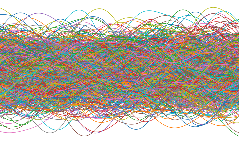
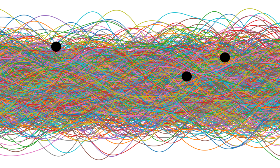
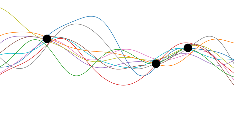
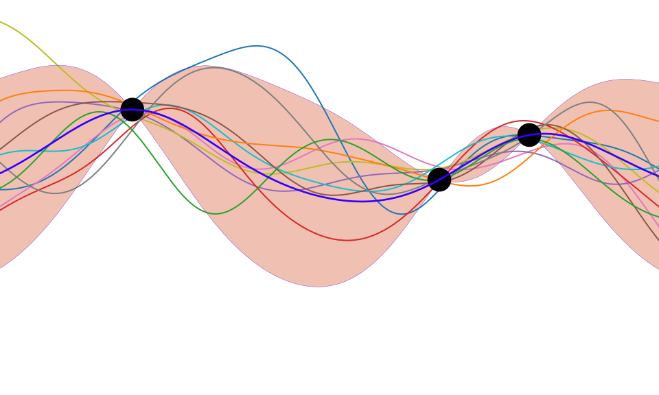
Emulation

Emulation

Emulation

Emulation

Emulation

Emulation
Deep Emulation

Deep Emulation

Deep Emulation

Emulation

Conclusion

  • AI is fundamentally ML System Design
  • We are not ready to deploy automation in uncontrolled environments.
  • Until we can monitoring and update will be key.

Thanks!

References