The Future of AI
Systems, Data Science, Biology, Medicine
Autumn Data Science School, Cambridge
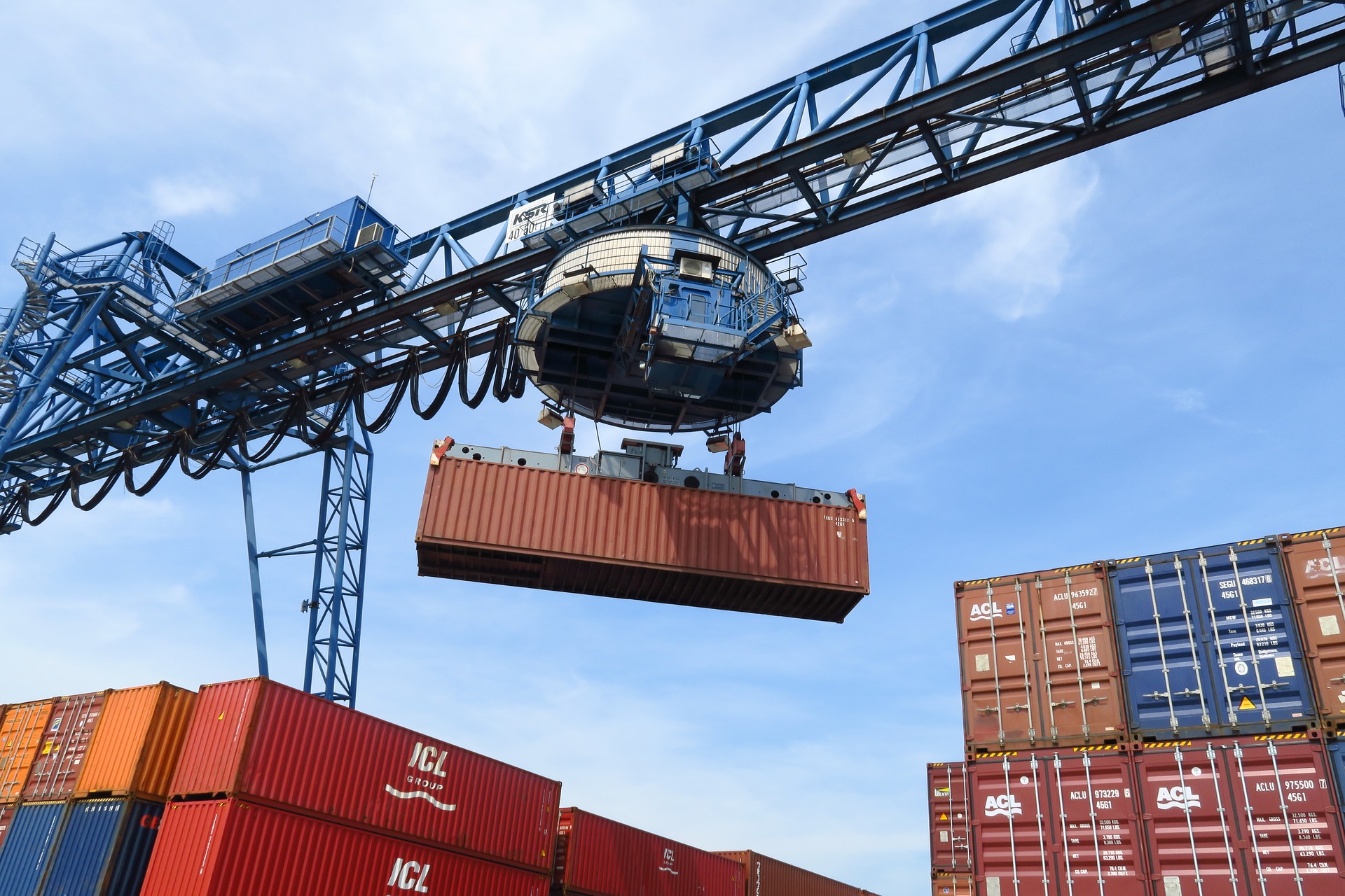
Supply Chain
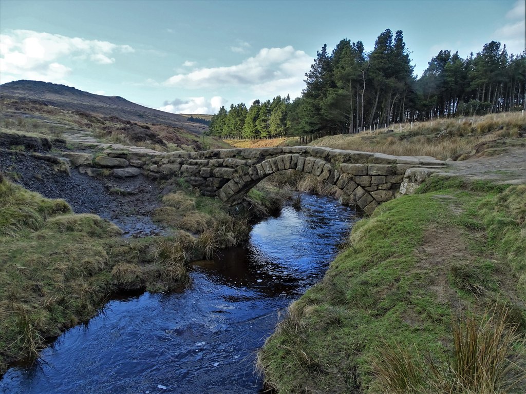
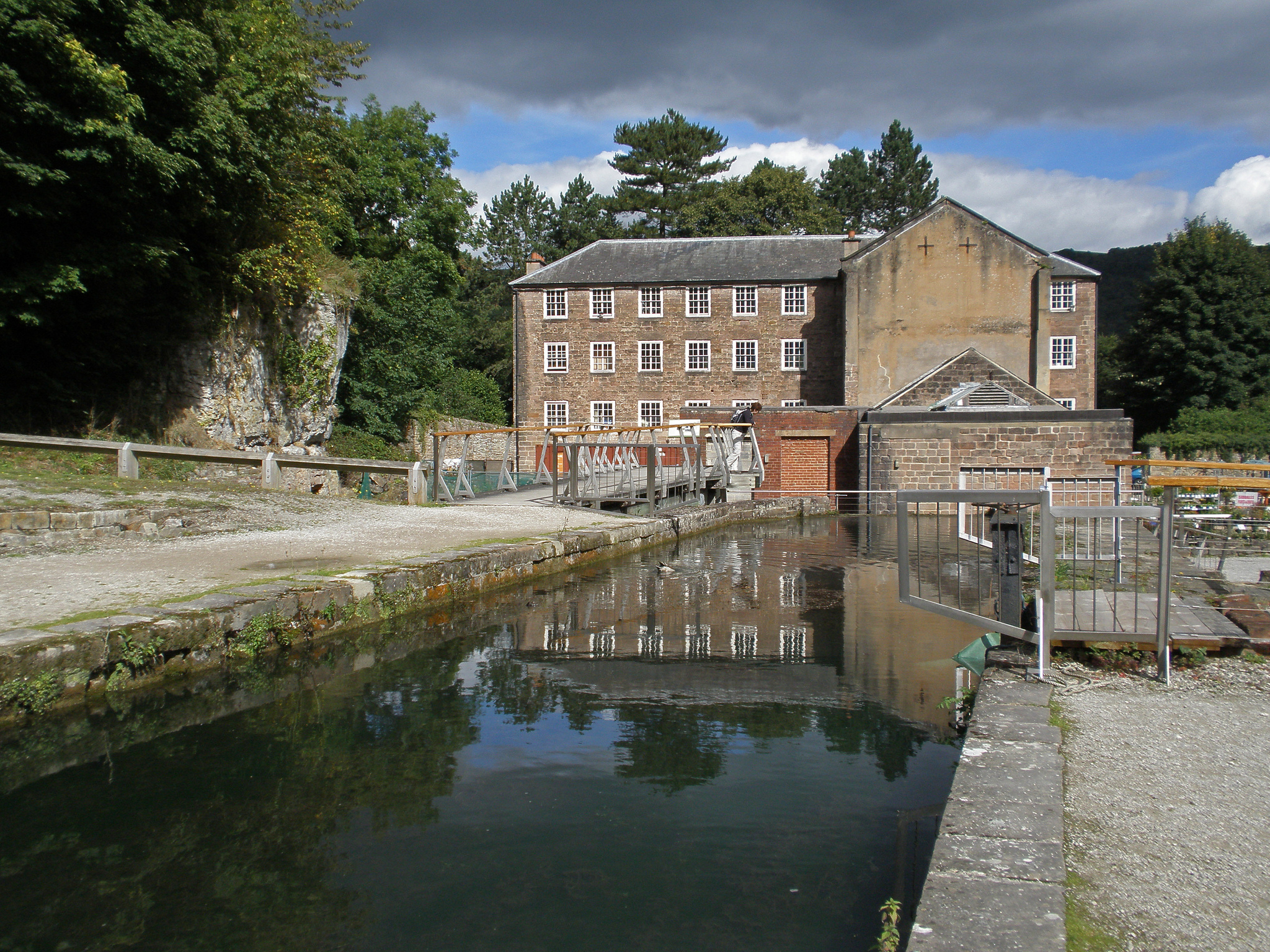
Cromford
Deep Freeze

Deep Freeze
DeepFace
Outline of the DeepFace architecture. A front-end of a single convolution-pooling-convolution filtering on the rectified input, followed by three locally-connected layers and two fully-connected layers. Color illustrates feature maps produced at each layer. The net includes more than 120 million parameters, where more than 95% come from the local and fully connected.
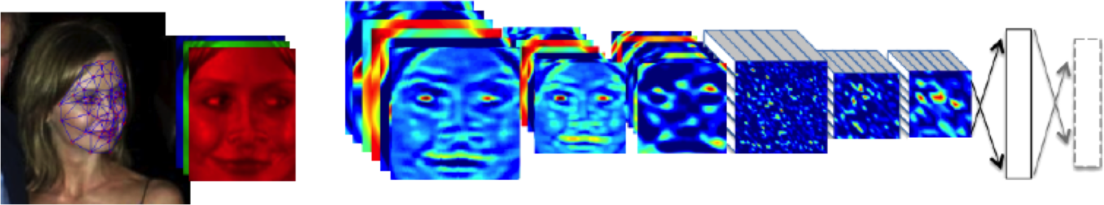
Source: DeepFace (Taigman et al., 2014)
Deep Learning as Pinball
Olympic Marathon Data
|
|
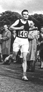
Alan Turing
|
|
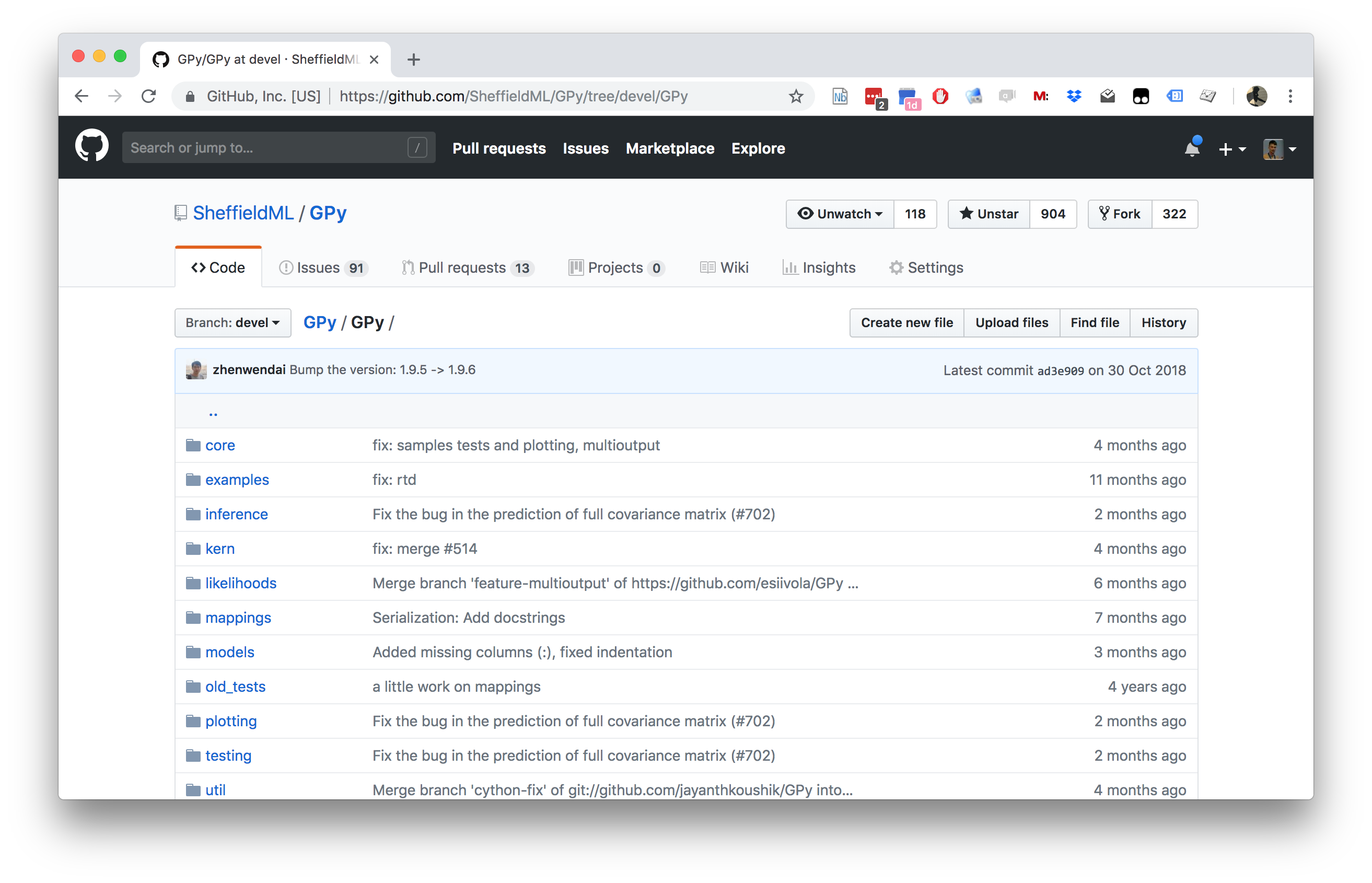
GPy: A Gaussian Process Framework in Python

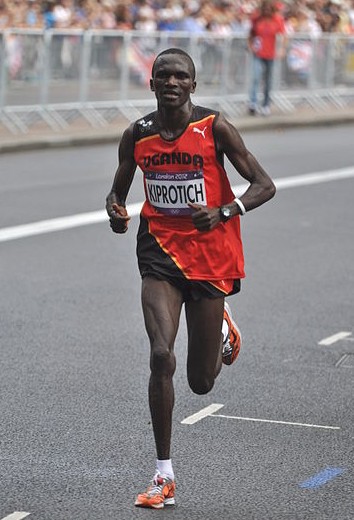
Example: Prediction of Malaria Incidence in Uganda
- Work with Ricardo Andrade Pacheco, John Quinn and Martin Mubaganzi (Makerere University, Uganda)
- See AI-DEV Group.
Malaria Prediction in Uganda
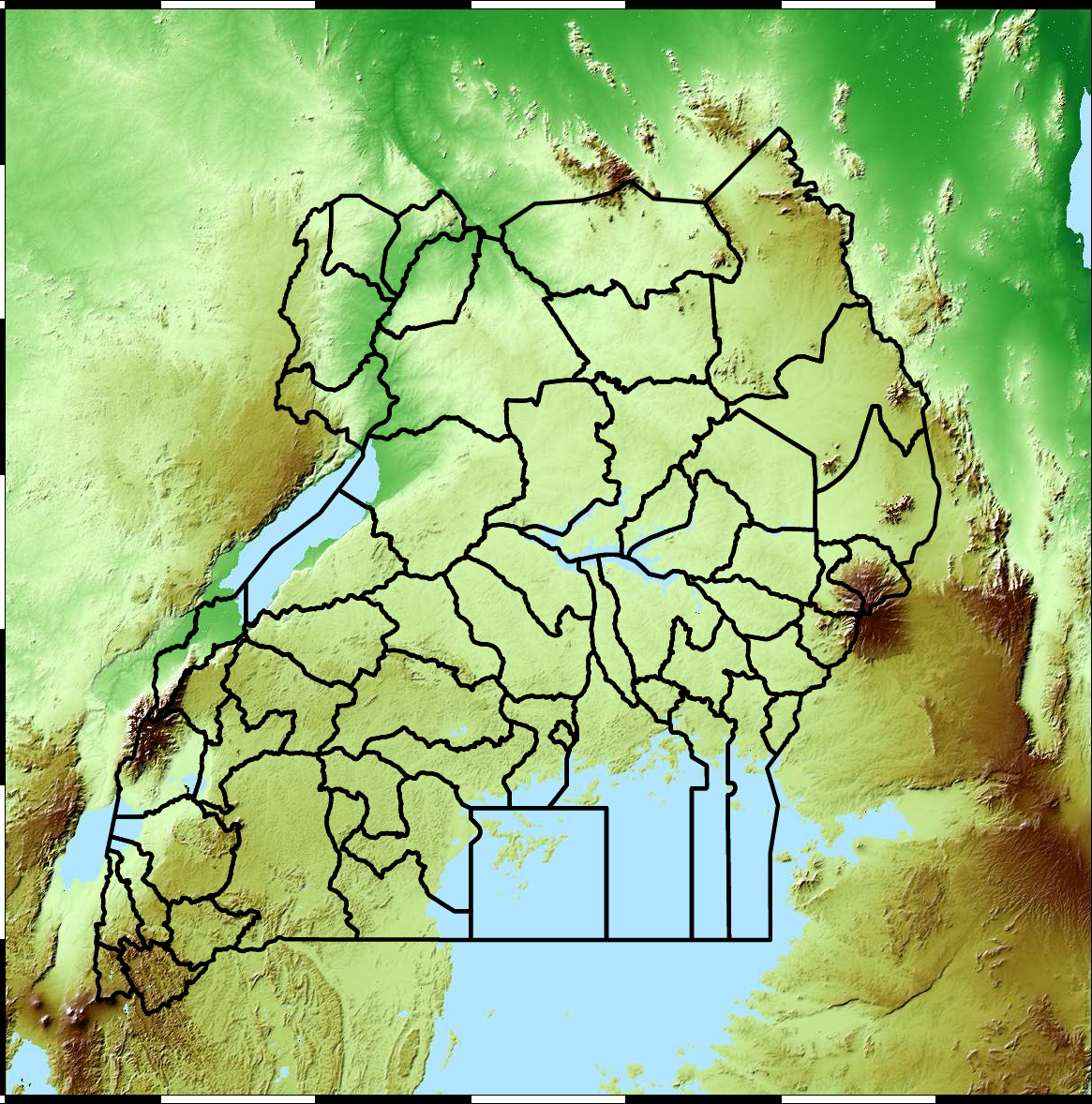
(Andrade-Pacheco et al., 2014; Mubangizi et al., 2014)
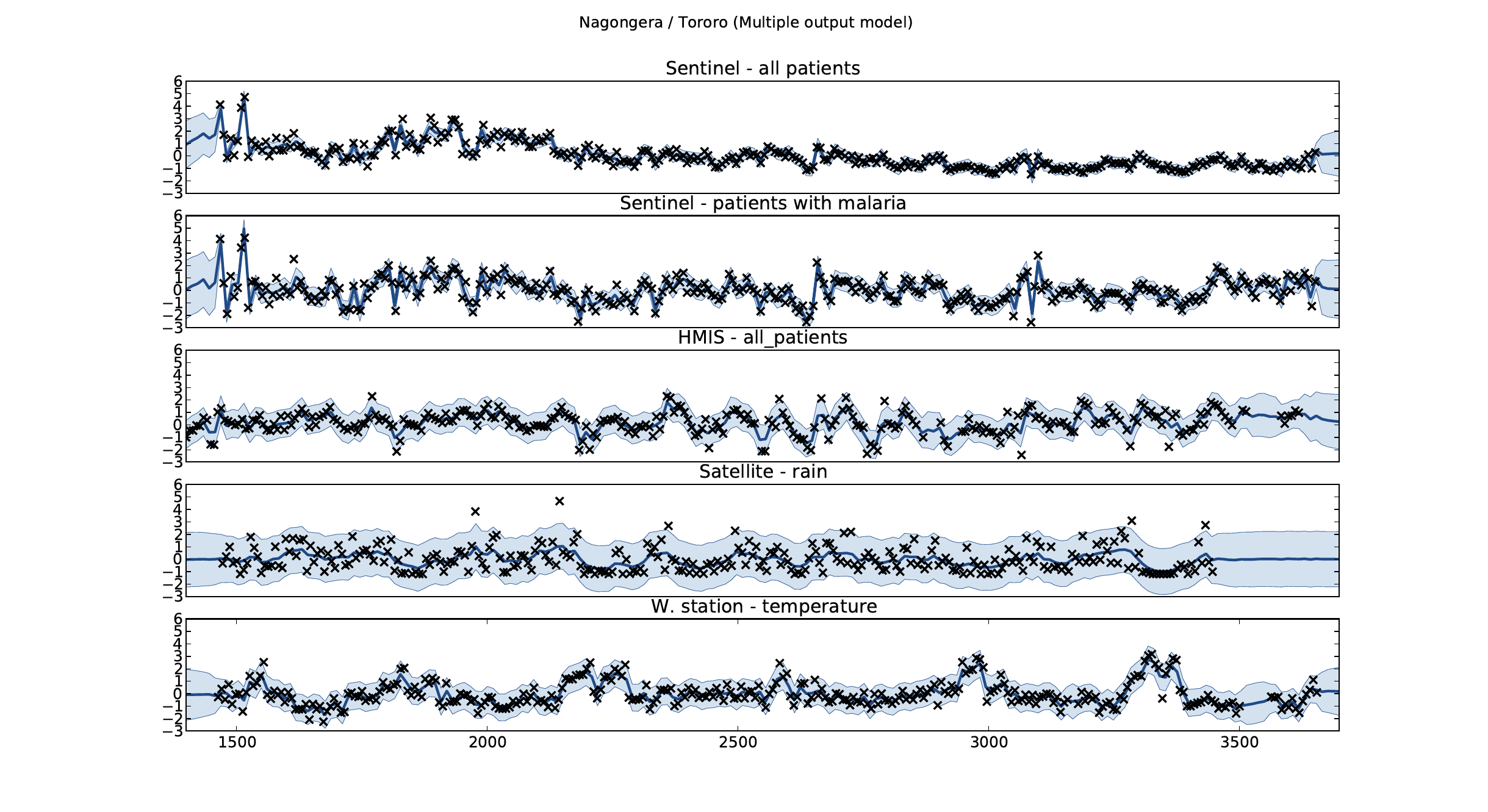
Malaria Prediction in Nagongera (Sentinel Site)
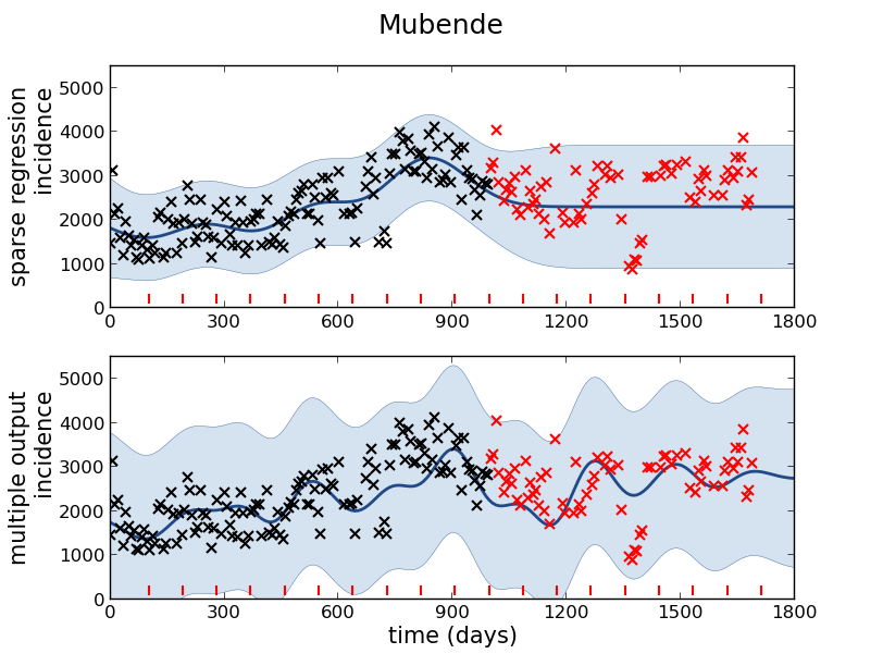
Malaria Prediction in Uganda
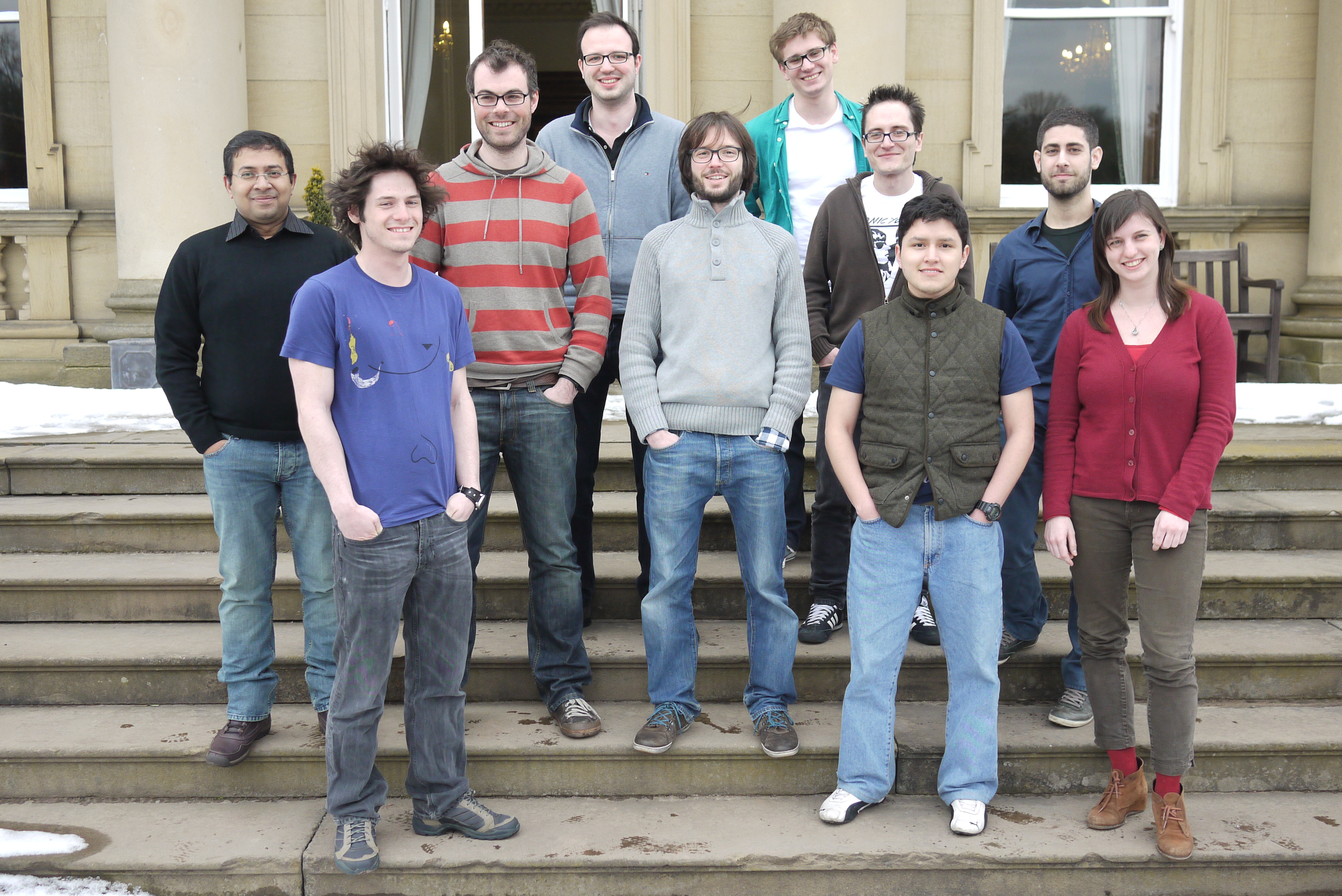
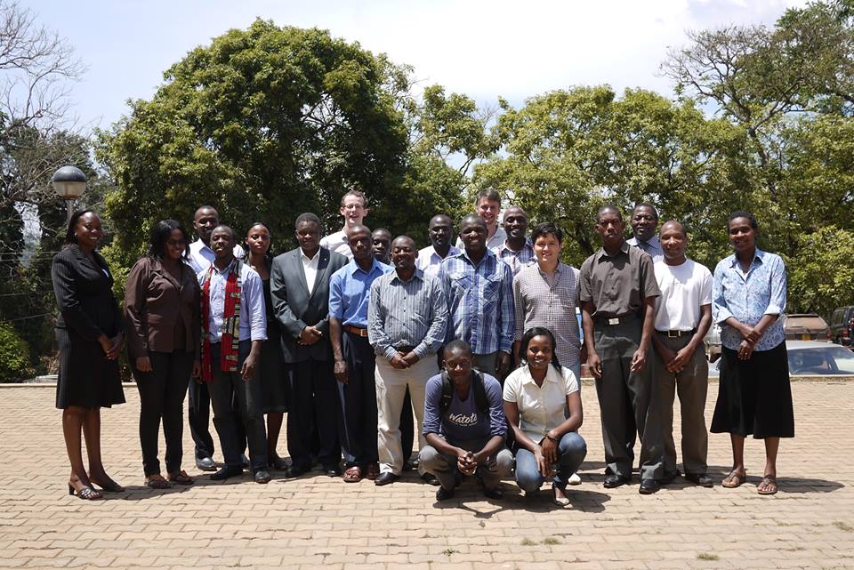
GP School at Makerere
Early Warning System
Early Warning Systems