Naive Days
Challenges Before the AI Revolution Arrives
University of Sheffield
There are three types of lies: lies, damned lies and statistics
??
There are three types of lies: lies, damned lies and statistics
Benjamin Disraeli
There are three types of lies: lies, damned lies and statistics
Benjamin Disraeli 1804-1881
There are three types of lies: lies, damned lies and ‘big data’
Neil Lawrence 1972-?
Mathematical Statistics
‘Mathematical Data Science’

What is Machine Learning?
\[ \text{data} + \text{model} \xrightarrow{\text{compute}} \text{prediction}\]
- data : observations, could be actively or passively acquired (meta-data).
- model : assumptions, based on previous experience (other data! transfer learning etc), or beliefs about the regularities of the universe. Inductive bias.
- prediction : an action to be taken or a categorization or a quality score.
- Royal Society Report: Machine Learning: Power and Promise of Computers that Learn by Example
What is Machine Learning?
\[\text{data} + \text{model} \xrightarrow{\text{compute}} \text{prediction}\]
- To combine data with a model need:
- a prediction function \(\mappingFunction (\cdot)\) includes our beliefs about the regularities of the universe
- an objective function \(\errorFunction (\cdot)\) defines the cost of misprediction.
Machine Learning
- Driver of two different domains:
- Data Science: arises from the fact that we now capture data by happenstance.
- Artificial Intelligence: emulation of human behaviour.
- Connection: Internet of Things
Machine Learning
- Driver of two different domains:
- Data Science: arises from the fact that we now capture data by happenstance.
- Artificial Intelligence: emulation of human behaviour.
- Connection: Internet of
Things
Machine Learning
- Driver of two different domains:
- Data Science: arises from the fact that we now capture data by happenstance.
- Artificial Intelligence: emulation of human behaviour.
- Connection: Internet of People
What does Machine Learning do?
- ML Automates through Data
- Strongly related to statistics.
- Field underpins revolution in data science and AI
- With AI:
- logic, robotics, computer vision, speech
- With Data Science:
- databases, data mining, statistics, visualization
What does Machine Learning do?
- Automation scales by codifying processes and automating them.
- Need:
- Interconnected components
- Compatible components
- Early examples:
- cf Colt 45, Ford Model T
Codify Through Mathematical Functions
- How does machine learning work?
- Jumper (jersey/sweater) purchase with logistic regression
\[ \text{odds} = \frac{p(\text{bought})}{p(\text{not bought})} \]
\[ \log \text{odds} = \beta_0 + \beta_1 \text{age} + \beta_2 \text{latitude}.\]
Codify Through Mathematical Functions
- How does machine learning work?
- Jumper (jersey/sweater) purchase with logistic regression
\[ p(\text{bought}) = \sigmoid{\beta_0 + \beta_1 \text{age} + \beta_2 \text{latitude}}.\]
Codify Through Mathematical Functions
- How does machine learning work?
- Jumper (jersey/sweater) purchase with logistic regression
\[ p(\text{bought}) = \sigmoid{\boldsymbol{\beta}^\top \inputVector}.\]
Codify Through Mathematical Functions
- How does machine learning work?
- Jumper (jersey/sweater) purchase with logistic regression
\[ \dataScalar = \mappingFunction\left(\inputVector, \boldsymbol{\beta}\right).\]
We call \(\mappingFunction(\cdot)\) the prediction function.
Fit to Data
- Use an objective function
\[\errorFunction(\boldsymbol{\beta}, \dataMatrix, \inputMatrix)\]
- E.g. least squares \[\errorFunction(\boldsymbol{\beta}, \dataMatrix, \inputMatrix) = \sum_{i=1}^\numData \left(\dataScalar_i - \mappingFunction(\inputVector_i, \boldsymbol{\beta})\right)^2.\]
Two Components
- Prediction function, \(\mappingFunction(\cdot)\)
- Objective function, \(\errorFunction(\cdot)\)
Deep Learning
These are interpretable models: vital for disease etc.
Modern machine learning methods are less interpretable
Example: face recognition
Deep Learning
These are interpretable models: vital for disease modeling etc.
Modern machine learning methods are less interpretable
Example: face recognition
DeepFace
Outline of the DeepFace architecture. A front-end of a single convolution-pooling-convolution filtering on the rectified input, followed by three locally-connected layers and two fully-connected layers. Color illustrates feature maps produced at each layer. The net includes more than 120 million parameters, where more than 95% come from the local and fully connected.
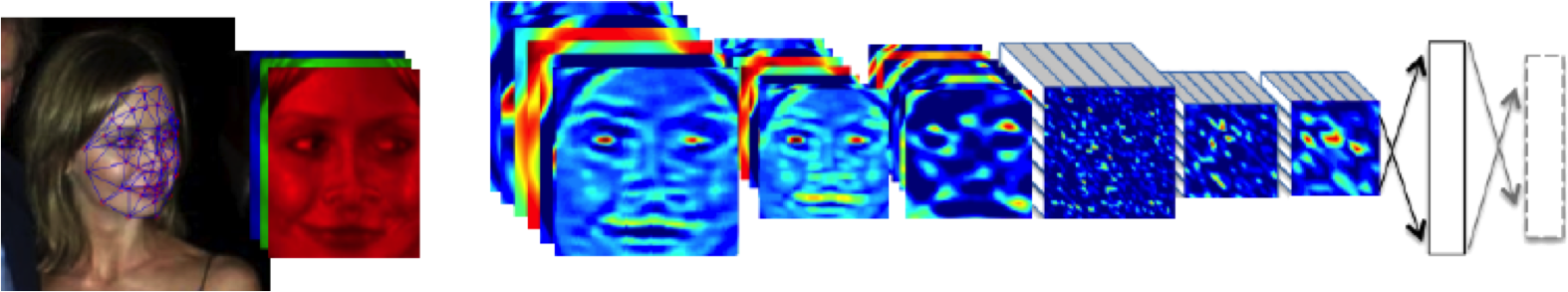
Source: DeepFace (Taigman et al., 2014)
Deep Learning as Pinball

From Model to Decision

|
\[\text{data} + \text{model} \xrightarrow{\text{compute}} \text{prediction}\] |
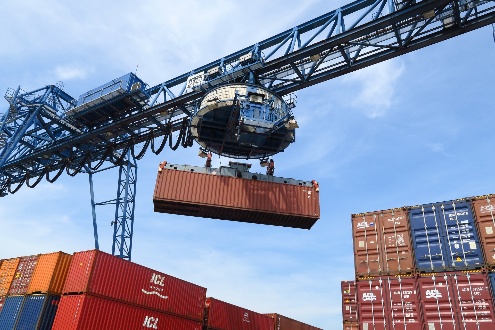
Machine Learning in Supply Chain
- Supply chain: Large Automated Decision Making Network
- Major Challenge:
- We have a mechanistic understanding of supply chain.
- Machine learning is a data driven technology.
Motto
Solve Supply Chain, then solve everything else.
Supply Chain
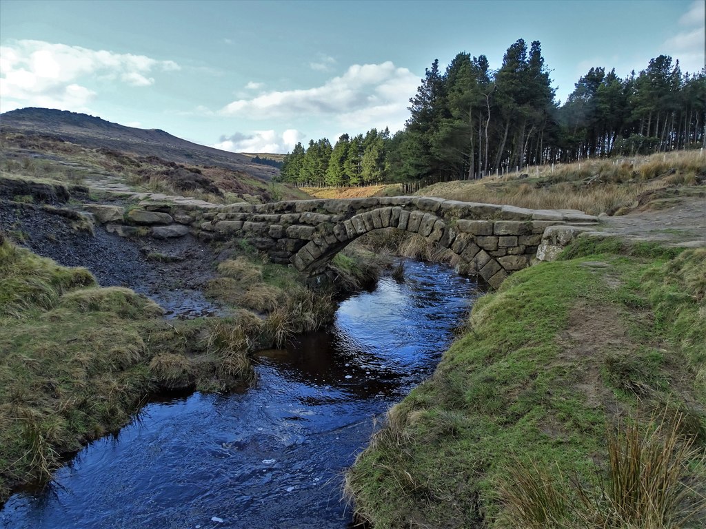
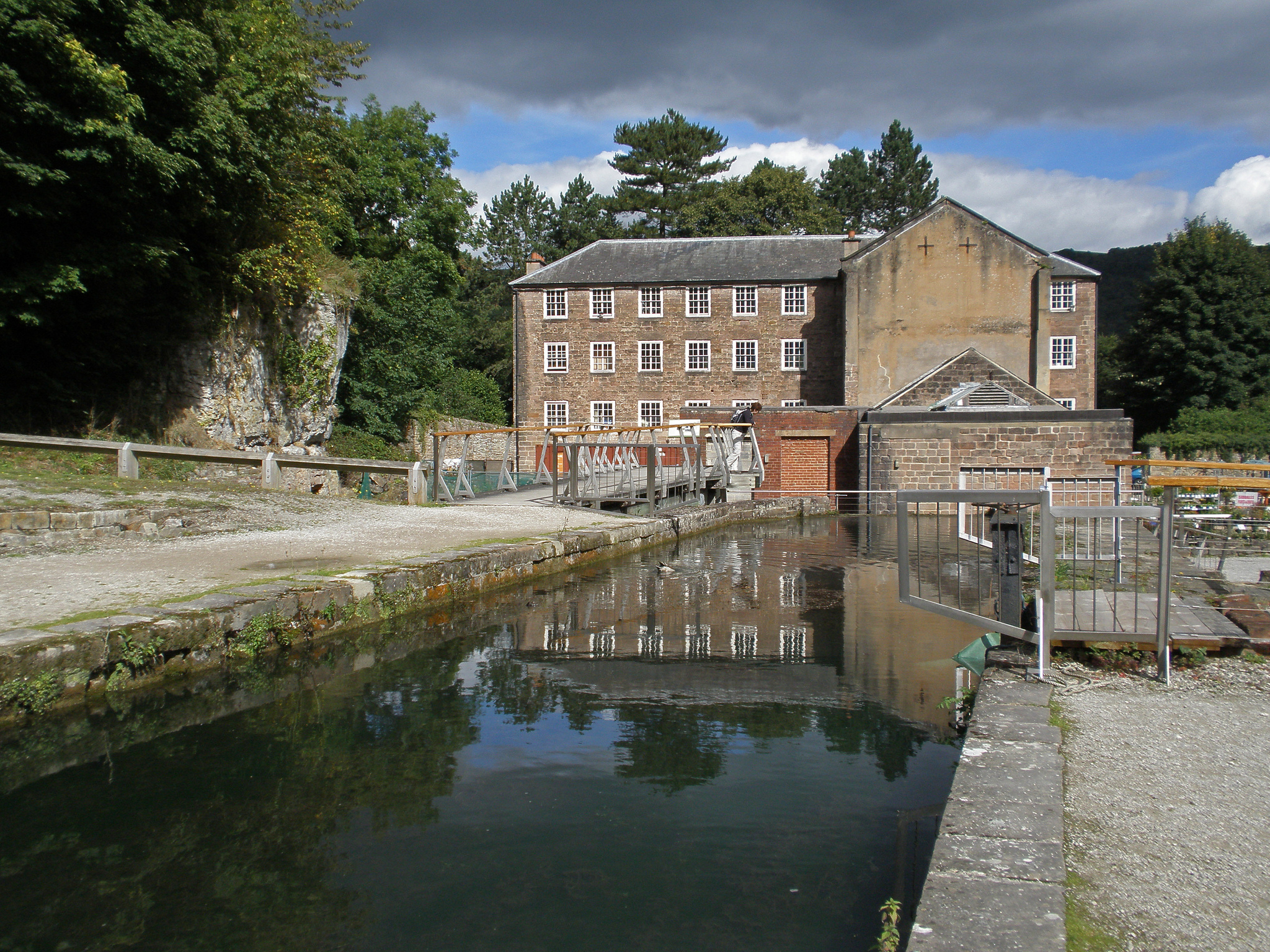
Cromford
Deep Freeze

Deep Freeze
SafeBoda

SafeBoda
With road accidents set to match HIV/AIDS as the highest cause of death in low/middle income countries by 2030, SafeBoda’s aim is to modernise informal transportation and ensure safe access to mobility.
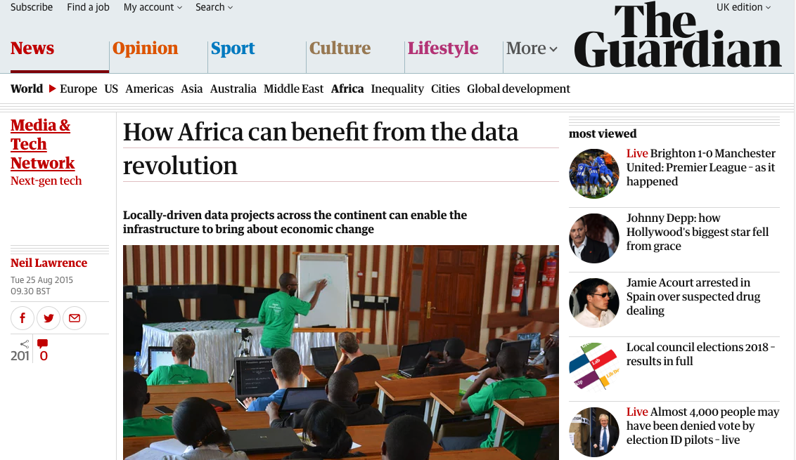
Data Science Africa is a bottom up initiative for capacity building in data science, machine learning and AI on the African continent
Example: Prediction of Malaria Incidence in Uganda
- Work with Ricardo Andrade Pacheco, John Quinn and Martin Mubaganzi (Makerere University, Uganda)
- See AI-DEV Group.
Malaria Prediction in Uganda
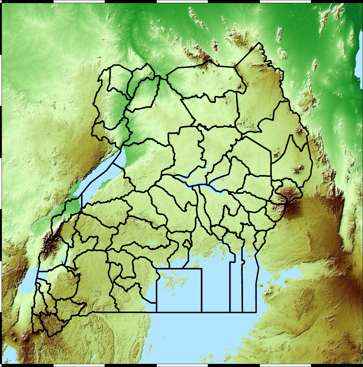
(Andrade-Pacheco et al., 2014; Mubangizi et al., 2014)
Tororo District
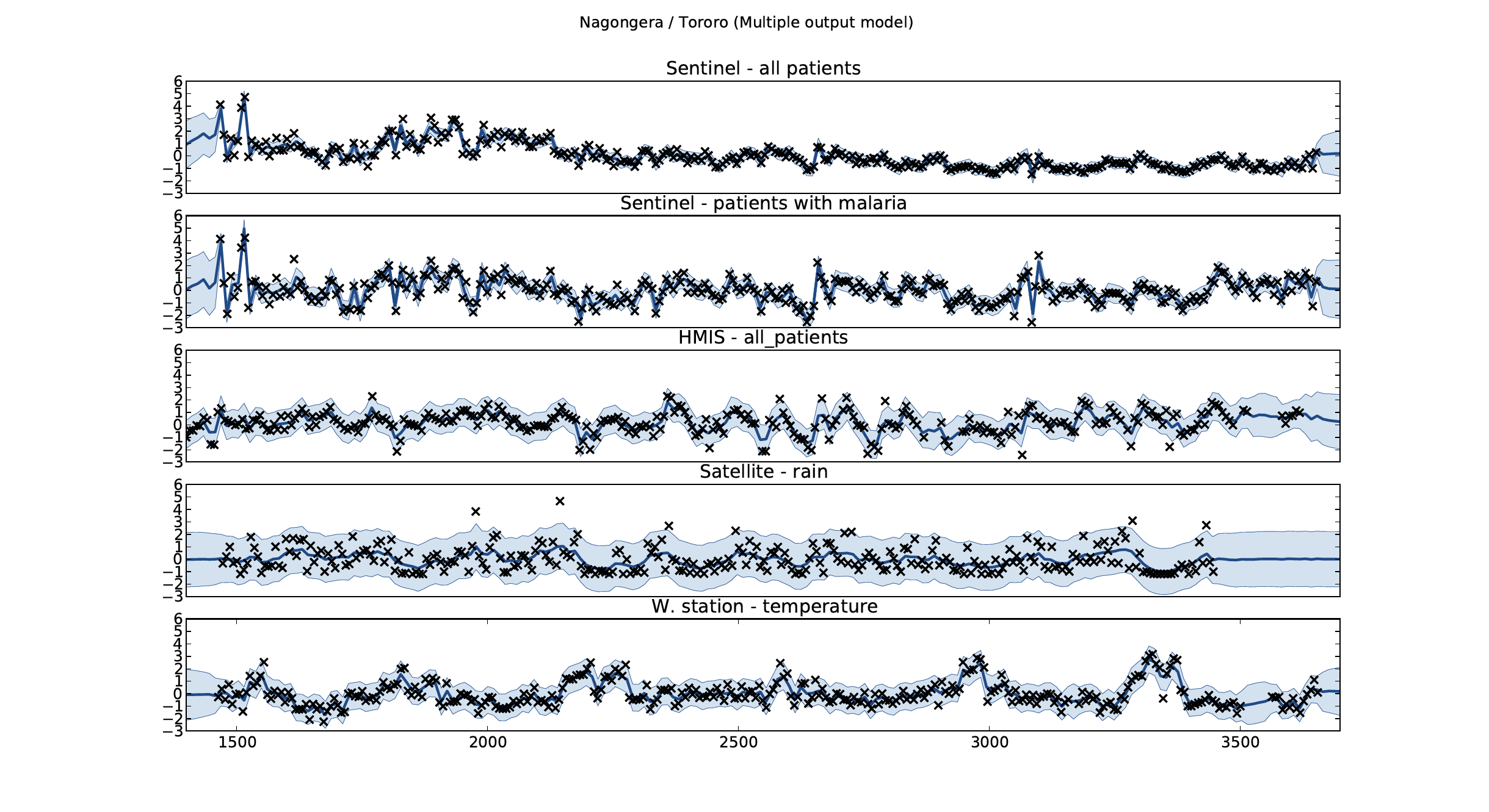
Malaria Prediction in Nagongera (Sentinel Site)
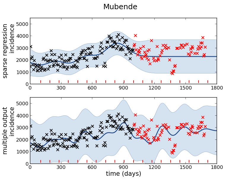
Mubende District
Malaria Prediction in Uganda
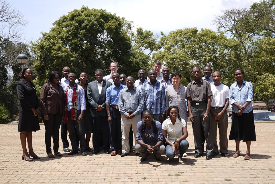
GP School at Makerere
Kabarole District
Early Warning System
Early Warning Systems
Deployment
Premise
Our machine learning is based on a software systems view that is 20 years out of date.
Continuous Deployment
- Deployment of modeling code.
- Data dependent models in production need continuous monitoring.
- Continous monitoring implies statistical tests rather than classic software tests.
You can also check my
Continuous Monitoring
- Continuous deployment:
- We’ve changed the code, we should test the effect.
- Continuous Monitoring:
- The world around us is changing, we should monitor the effect.
- Update our notions of testing: progression testing
Data Oriented Architectures
- Convert data to a first-class citizen.
- View system as operations on data streams.
- Expose data operations in a programmatic way.
Data Orientated Architectures
- Historically we’ve been software first
- A necessary but not sufficient condition for data first
- Move from
- service orientated architectures
- data orientated architectures
Streaming System
- Move from pull updates to push updates.
- Operate on rows rather than columns.
- Lead to stateless logic: persistence handled by system.
- Example Apache Kafka + Apache Flink
Streaming Architectures
- AWS Kinesis, Apache Kafka
- Not just about streaming
- Nodes in the architecture are stateless
- They persist through storing state on streams
- This brings the data inside out
Apache Flink
- Streams and transformations
- a stream is a (potentially never-ending) flow of data records
- a transformation: streams as input, produces transformed streams as output
Join
stream.join(otherStream)
    .where(<KeySelector>)
    .equalTo(<KeySelector>)
    .window(<WindowAssigner>)
    .apply(<JoinFunction>)
Milan
- Data Oriented Programming Language and runtime.
- DSL Embedded in Scala converts to an intermediate langugage.
- Intermediate language for compilation on different platforms (currently Flink)
Trading System
- High frequency share trading.
- Stream of prices with millisecond updates.
- Trades required on millisecond time line
Real Price
Future Price
Hypothetical Streams
- Real stream — share prices
- derived hypothetical stream — share prices in future.
- Hypothetical constrained by
- input constraints.
- decision functional
- computational requirements (latency)
Hypothetical Advantage
- Modelling is now required.
- But modelling is declared in the ecosystem.
- If it’s manual, warnings can be used
- calibration, fairness, dataset shift
- Opens door to Auto AI.
Ride Allocation Prediction
Ride Sharing: Service Oriented
Ride Sharing: Data Oriented
Ride Sharing: Hypothetical
Information Dynamics
- Potential for information feedback loops.
- Hypothetical streams are instantiated.
- Nature hypothesis (e.g. price prediction) can effect reality.
- Leads to information dynamics, similar to dynamics of governors.
- See e.g. Closed Loop Data Science at Glasgow.
Conclusions
- Challenge is in data and model ecosystem.
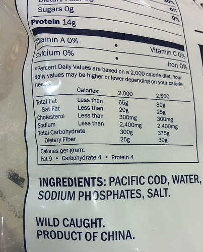
- Also problems of
- data quality (see e.g. Lawrence (2017)) and
- data sharing (article on
and Delacroix and Lawrence (2019)) * Physical systems can be easier to deploy becaue they’re contained.
Thanks!
- twitter: @lawrennd
- podcast: The Talking Machines
Guardian article on How African can benefit from the data revolution
Guardian article on Data Trusts
Blog post on Lies, Damned Lies and Big Data
Blog post on What is Machine Learning?
Blog post on Data Science as Debugging
References
Andrade-Pacheco, R., Mubangizi, M., Quinn, J., Lawrence, N.D., 2014. Consistent mapping of government malaria records across a changing territory delimitation. Malaria Journal 13. https://doi.org/10.1186/1475-2875-13-S1-P5
Delacroix, S., Lawrence, N.D., 2019. Bottom-up data trusts: Disturbing the “one size fits all” approach to data governance. International Data Privacy Law. https://doi.org/10.1093/idpl/ipz014
Lawrence, N.D., 2017. Data readiness levels. arXiv.
Mubangizi, M., Andrade-Pacheco, R., Smith, M.T., Quinn, J., Lawrence, N.D., 2014. Malaria surveillance with multiple data sources using Gaussian process models, in: 1st International Conference on the Use of Mobile ICT in Africa.
Taigman, Y., Yang, M., Ranzato, M., Wolf, L., 2014. DeepFace: Closing the gap to human-level performance in face verification, in: Proceedings of the IEEE Computer Society Conference on Computer Vision and Pattern Recognition. https://doi.org/10.1109/CVPR.2014.220