Deep GPs

Deep Gaussian Processes

GPy: A Gaussian Process Framework in Python

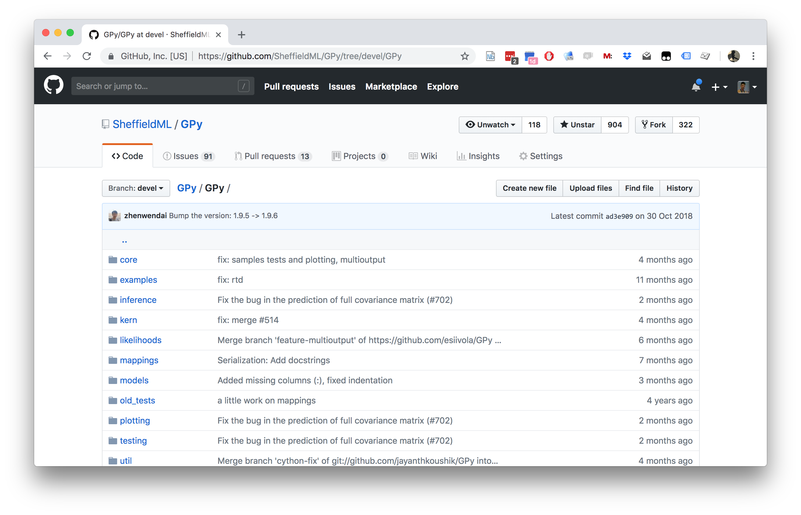
GPy: A Gaussian Process Framework in Python

• BSD Licensed software base.
• Wide availability of libraries, ‘modern’ scripting language.
• Allows us to set projects to undergraduates in Comp Sci that use GPs.
• Available through GitHub https://github.com/SheffieldML/GPy
• Reproducible Research with Jupyter Notebook.

Features

• Probabilistic-style programming (specify the model, not the algorithm).
• Non-Gaussian likelihoods.
• Multivariate outputs.
• Dimensionality reduction.
• Approximations for large data sets.

Low Rank Gaussian Processes

Approximations

Approximations

Approximations

Approximations

Low Rank Motivation

• Inference in a GP has the following demands:

  Complexity:	\(\mathcal{O}(n^3)\)
  Storage:	\(\mathcal{O}(n^2)\)

• Inference in a low rank GP has the following demands:

  Complexity:	\(\mathcal{O}(nm^2)\)
  Storage:	\(\mathcal{O}(nm)\)

  where \(m\) is a user chosen parameter.

Snelson and Ghahramani (n.d.),Quiñonero Candela and Rasmussen (2005),Lawrence (n.d.),Titsias (n.d.),Bui et al. (2017)

Variational Compression

• Inducing variables are a compression of the real observations.
• They are like pseudo-data. They can be in space of \(\mathbf{ f}\) or a space that is related through a linear operator (Álvarez et al., 2010) — e.g. a gradient or convolution.

Variational Compression II

• Introduce inducing variables.
• Compress information into the inducing variables and avoid the need to store all the data.
• Allow for scaling e.g. stochastic variational Hensman et al. (n.d.) or parallelization Gal et al. (n.d.),Dai et al. (2014), Seeger et al. (2017)

Nonparametric Gaussian Processes

• We’ve seen how we go from parametric to non-parametric.

• The limit implies infinite dimensional \(\mathbf{ w}\).

• Gaussian processes are generally non-parametric: combine data with covariance function to get model.

• This representation cannot be summarized by a parameter vector of a fixed size.

The Parametric Bottleneck

• Parametric models have a representation that does not respond to increasing training set size.

• Bayesian posterior distributions over parameters contain the information about the training data.

  • Use Bayes’ rule from training data, \(p\left(\mathbf{ w}|\mathbf{ y}, \mathbf{X}\right)\),

  • Make predictions on test data \[p\left(y_*|\mathbf{X}_*, \mathbf{ y}, \mathbf{X}\right) = \int p\left(y_*|\mathbf{ w},\mathbf{X}_*\right)p\left(\mathbf{ w}|\mathbf{ y}, \mathbf{X})\text{d}\mathbf{ w}\right).\]

• \(\mathbf{ w}\) becomes a bottleneck for information about the training set to pass to the test set.

• Solution: increase \(m\) so that the bottleneck is so large that it no longer presents a problem.

• How big is big enough for \(m\)? Non-parametrics says \(m\rightarrow \infty\).

The Parametric Bottleneck

• Now no longer possible to manipulate the model through the standard parametric form.

Making Predictions

• For non-parametrics prediction at new points \(\mathbf{ f}_*\) is made by conditioning on \(\mathbf{ f}\) in the joint distribution.

Augment Variable Space

• Augment variable space with inducing observations, \(\mathbf{ u}\) \[ \begin{bmatrix} \mathbf{ f}\\ \mathbf{ u} \end{bmatrix} \sim \mathcal{N}\left(\mathbf{0},\mathbf{K}\right) \] with \[ \mathbf{K}= \begin{bmatrix} \mathbf{K}_{\mathbf{ f}\mathbf{ f}}& \mathbf{K}_{\mathbf{ f}\mathbf{ u}}\\ \mathbf{K}_{\mathbf{ u}\mathbf{ f}}& \mathbf{K}_{\mathbf{ u}\mathbf{ u}} \end{bmatrix} \]

Joint Density

\[ p(\mathbf{ f}, \mathbf{ u}) = p(\mathbf{ f}| \mathbf{ u}) p(\mathbf{ u}) \] to augment our model \[ y(\mathbf{ x}) = f(\mathbf{ x}) + \epsilon, \] giving \[ p(\mathbf{ y}) = \int p(\mathbf{ y}|\mathbf{ f}) p(\mathbf{ f}) \text{d}\mathbf{ f}, \] where for the independent case we have \(p(\mathbf{ y}| \mathbf{ f}) = \prod_{i=1}^np(y_i|f_i)\).

Auxilliary Variables

\[ p(\mathbf{ y}) = \int p(\mathbf{ y}|\mathbf{ f}) p(\mathbf{ f}|\mathbf{ u}) p(\mathbf{ u}) \text{d}\mathbf{ u}\text{d}\mathbf{ f}. \] Integrating over \(\mathbf{ f}\) \[ p(\mathbf{ y}) = \int p(\mathbf{ y}|\mathbf{ u}) p(\mathbf{ u}) \text{d}\mathbf{ u}. \]

Parametric Comparison

\[ y(\mathbf{ x}) = \mathbf{ w}^\top\boldsymbol{ \phi}(\mathbf{ x}) + \epsilon \]

\[ p(\mathbf{ y}) = \int p(\mathbf{ y}|\mathbf{ w}) p(\mathbf{ w}) \text{d} \mathbf{ w} \]

\[ p(\mathbf{ y}^*|\mathbf{ y}) = \int p(\mathbf{ y}^*|\mathbf{ w}) p(\mathbf{ w}|\mathbf{ y}) \text{d} \mathbf{ w} \]

New Form

\[ p(\mathbf{ y}^*|\mathbf{ y}) = \int p(\mathbf{ y}^*|\mathbf{ u}) p(\mathbf{ u}|\mathbf{ y}) \text{d} \mathbf{ u} \]

• but \(\mathbf{ u}\) is not a parameter

• Unfortunately computing \(p(\mathbf{ y}|\mathbf{ u})\) is intractable

Variational Bound on \(p(\mathbf{ y}|\mathbf{ u})\)

\[ \begin{aligned} \log p(\mathbf{ y}|\mathbf{ u}) & = \log \int p(\mathbf{ y}|\mathbf{ f}) p(\mathbf{ f}|\mathbf{ u}) \text{d}\mathbf{ f}\\ & = \int q(\mathbf{ f}) \log \frac{p(\mathbf{ y}|\mathbf{ f}) p(\mathbf{ f}|\mathbf{ u})}{q(\mathbf{ f})}\text{d}\mathbf{ f}+ \text{KL}\left( q(\mathbf{ f})\,\|\,p(\mathbf{ f}|\mathbf{ y}, \mathbf{ u}) \right). \end{aligned} \]

Choose form for \(q(\cdot)\)

• Set \(q(\mathbf{ f})=p(\mathbf{ f}|\mathbf{ u})\), \[ \log p(\mathbf{ y}|\mathbf{ u}) \geq \int p(\mathbf{ f}|\mathbf{ u}) \log p(\mathbf{ y}|\mathbf{ f})\text{d}\mathbf{ f}. \] \[ p(\mathbf{ y}|\mathbf{ u}) \geq \exp \int p(\mathbf{ f}|\mathbf{ u}) \log p(\mathbf{ y}|\mathbf{ f})\text{d}\mathbf{ f}. \] (Titsias, n.d.)

Optimal Compression in Inducing Variables

• Maximizing lower bound minimizes the KL divergence (information gain): \[ \text{KL}\left( p(\mathbf{ f}|\mathbf{ u})\,\|\,p(\mathbf{ f}|\mathbf{ y}, \mathbf{ u}) \right) = \int p(\mathbf{ f}|\mathbf{ u}) \log \frac{p(\mathbf{ f}|\mathbf{ u})}{p(\mathbf{ f}|\mathbf{ y}, \mathbf{ u})}\text{d}\mathbf{ u} \]

• This is minimized when the information stored about \(\mathbf{ y}\) is stored already in \(\mathbf{ u}\).

• The bound seeks an optimal compression from the information gain perspective.

• If \(\mathbf{ u}= \mathbf{ f}\) bound is exact (\(\mathbf{ f}\) \(d\)-separates \(\mathbf{ y}\) from \(\mathbf{ u}\)).

Choice of Inducing Variables

• Free to choose whatever heuristics for the inducing variables.
• Can quantify which heuristics perform better through checking lower bound.

\[ \begin{bmatrix} \mathbf{ f}\\ \mathbf{ u} \end{bmatrix} \sim \mathcal{N}\left(\mathbf{0},\mathbf{K}\right) \] with \[ \mathbf{K}= \begin{bmatrix} \mathbf{K}_{\mathbf{ f}\mathbf{ f}}& \mathbf{K}_{\mathbf{ f}\mathbf{ u}}\\ \mathbf{K}_{\mathbf{ u}\mathbf{ f}}& \mathbf{K}_{\mathbf{ u}\mathbf{ u}} \end{bmatrix} \]

Variational Compression

• Inducing variables are a compression of the real observations.
• They are like pseudo-data. They can be in space of \(\mathbf{ f}\) or a space that is related through a linear operator (Álvarez et al., 2010) — e.g. a gradient or convolution.

Variational Compression II

• Resulting algorithms reduce computational complexity.
• Also allow deployment of more standard scaling techniques.
• E.g. Stochastic variational inference Hoffman et al. (2012)
• Allow for scaling e.g. stochastic variational Hensman et al. (n.d.) or parallelization (Dai et al., 2014; Gal et al., n.d.; Seeger et al., 2017)

Full Gaussian Process Fit

Inducing Variable Fit

Inducing Variable Param Optimize

Inducing Variable Full Optimize

Eight Optimized Inducing Variables

Full Gaussian Process Fit

Modern Review

• A Unifying Framework for Gaussian Process Pseudo-Point Approximations using Power Expectation Propagation Bui et al. (2017)

• Deep Gaussian Processes and Variational Propagation of Uncertainty Damianou (2015)

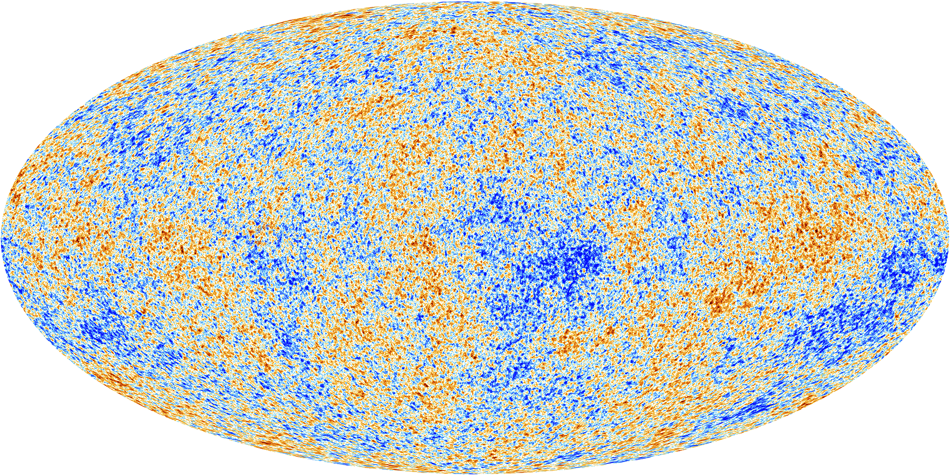
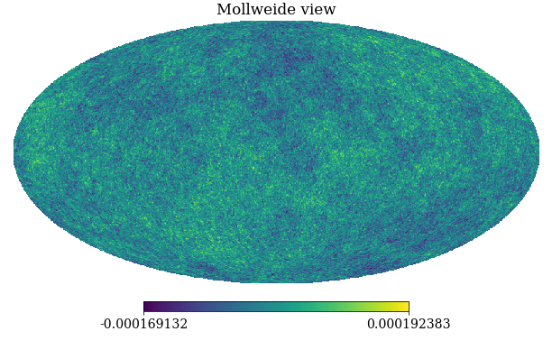
Structure of Priors

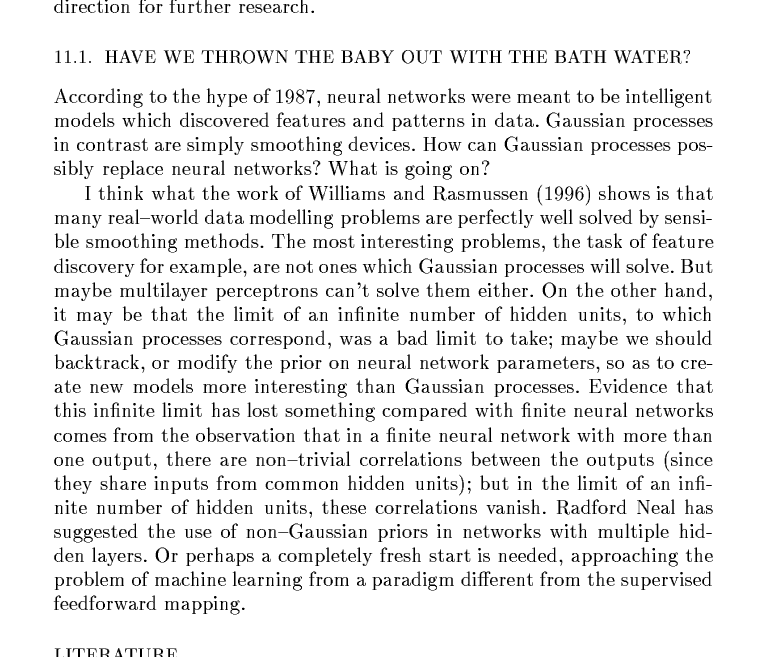
MacKay: NeurIPS Tutorial 1997 “Have we thrown out the baby with the bathwater?” (Published as MacKay, n.d.)

Deep Neural Network

Deep Neural Network

Mathematically

\[ \begin{align} \mathbf{ h}_{1} &= \phi\left(\mathbf{W}_1 \mathbf{ x}\right)\\ \mathbf{ h}_{2} &= \phi\left(\mathbf{W}_2\mathbf{ h}_{1}\right)\\ \mathbf{ h}_{3} &= \phi\left(\mathbf{W}_3 \mathbf{ h}_{2}\right)\\ \mathbf{ y}&= \mathbf{ w}_4 ^\top\mathbf{ h}_{3} \end{align} \]

Overfitting

• Potential problem: if number of nodes in two adjacent layers is big, corresponding \(\mathbf{W}\) is also very big and there is the potential to overfit.

• Proposed solution: “dropout”.

• Alternative solution: parameterize \(\mathbf{W}\) with its SVD. \[ \mathbf{W}= \mathbf{U}\boldsymbol{ \Lambda}\mathbf{V}^\top \] or \[ \mathbf{W}= \mathbf{U}\mathbf{V}^\top \] where if \(\mathbf{W}\in \Re^{k_1\times k_2}\) then \(\mathbf{U}\in \Re^{k_1\times q}\) and \(\mathbf{V}\in \Re^{k_2\times q}\), i.e. we have a low rank matrix factorization for the weights.

Low Rank Approximation

Bottleneck Layers in Deep Neural Networks

Deep Neural Network

Mathematically

The network can now be written mathematically as \[ \begin{align} \mathbf{ z}_{1} &= \mathbf{V}^\top_1 \mathbf{ x}\\ \mathbf{ h}_{1} &= \phi\left(\mathbf{U}_1 \mathbf{ z}_{1}\right)\\ \mathbf{ z}_{2} &= \mathbf{V}^\top_2 \mathbf{ h}_{1}\\ \mathbf{ h}_{2} &= \phi\left(\mathbf{U}_2 \mathbf{ z}_{2}\right)\\ \mathbf{ z}_{3} &= \mathbf{V}^\top_3 \mathbf{ h}_{2}\\ \mathbf{ h}_{3} &= \phi\left(\mathbf{U}_3 \mathbf{ z}_{3}\right)\\ \mathbf{ y}&= \mathbf{ w}_4^\top\mathbf{ h}_{3}. \end{align} \]

A Cascade of Neural Networks

\[ \begin{align} \mathbf{ z}_{1} &= \mathbf{V}^\top_1 \mathbf{ x}\\ \mathbf{ z}_{2} &= \mathbf{V}^\top_2 \phi\left(\mathbf{U}_1 \mathbf{ z}_{1}\right)\\ \mathbf{ z}_{3} &= \mathbf{V}^\top_3 \phi\left(\mathbf{U}_2 \mathbf{ z}_{2}\right)\\ \mathbf{ y}&= \mathbf{ w}_4 ^\top \mathbf{ z}_{3} \end{align} \]

Cascade of Gaussian Processes

• Replace each neural network with a Gaussian process \[ \begin{align} \mathbf{ z}_{1} &= \mathbf{ f}_1\left(\mathbf{ x}\right)\\ \mathbf{ z}_{2} &= \mathbf{ f}_2\left(\mathbf{ z}_{1}\right)\\ \mathbf{ z}_{3} &= \mathbf{ f}_3\left(\mathbf{ z}_{2}\right)\\ \mathbf{ y}&= \mathbf{ f}_4\left(\mathbf{ z}_{3}\right) \end{align} \]

• Equivalent to prior over parameters, take width of each layer to infinity.

Deep Learning

DeepFace

Outline of the DeepFace architecture. A front-end of a single convolution-pooling-convolution filtering on the rectified input, followed by three locally-connected layers and two fully-connected layers. Color illustrates feature maps produced at each layer. The net includes more than 120 million parameters, where more than 95% come from the local and fully connected.

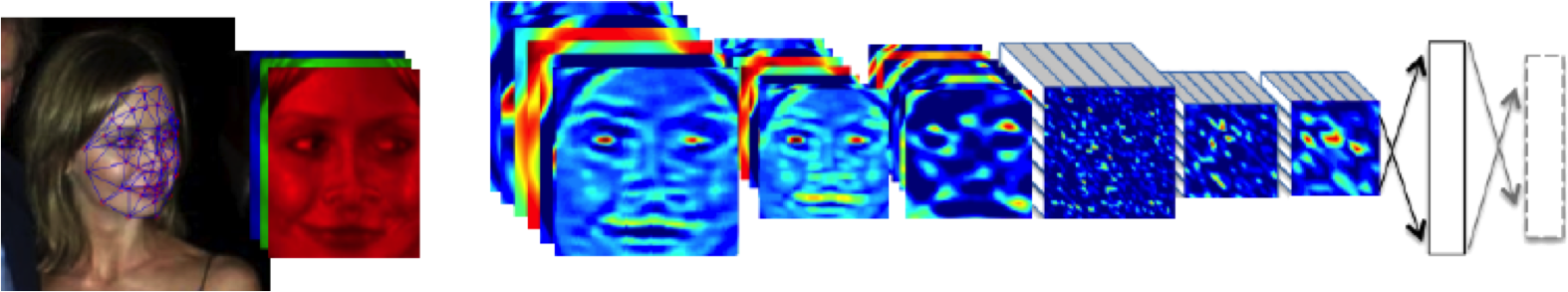
Source: DeepFace (Taigman et al., 2014)

Deep Learning as Pinball

Mathematically

• Composite multivariate function

  \[ \mathbf{g}(\mathbf{ x})=\mathbf{ f}_5(\mathbf{ f}_4(\mathbf{ f}_3(\mathbf{ f}_2(\mathbf{ f}_1(\mathbf{ x}))))). \]

Equivalent to Markov Chain

• Composite multivariate function \[ p(\mathbf{ y}|\mathbf{ x})= p(\mathbf{ y}|\mathbf{ f}_5)p(\mathbf{ f}_5|\mathbf{ f}_4)p(\mathbf{ f}_4|\mathbf{ f}_3)p(\mathbf{ f}_3|\mathbf{ f}_2)p(\mathbf{ f}_2|\mathbf{ f}_1)p(\mathbf{ f}_1|\mathbf{ x}) \]

Why Deep?

• Gaussian processes give priors over functions.

• Elegant properties:

  • e.g. Derivatives of process are also Gaussian distributed (if they exist).

• For particular covariance functions they are ‘universal approximators’, i.e. all functions can have support under the prior.

• Gaussian derivatives might ring alarm bells.

• E.g. a priori they don’t believe in function ‘jumps’.

Stochastic Process Composition

• From a process perspective: process composition.

• A (new?) way of constructing more complex processes based on simpler components.

Difficulty for Probabilistic Approaches

• Propagate a probability distribution through a non-linear mapping.

• Normalisation of distribution becomes intractable.

Difficulty for Probabilistic Approaches

• Propagate a probability distribution through a non-linear mapping.

• Normalisation of distribution becomes intractable.

Difficulty for Probabilistic Approaches

• Propagate a probability distribution through a non-linear mapping.

• Normalisation of distribution becomes intractable.

Standard Variational Approach Fails

• Standard variational bound has the form: \[ \mathcal{L}= \left<\log p(\mathbf{ y}|\mathbf{Z})\right>_{q(\mathbf{Z})} + \text{KL}\left( q(\mathbf{Z})\,\|\,p(\mathbf{Z}) \right) \]

Standard Variational Approach Fails

• Requires expectation of \(\log p(\mathbf{ y}|\mathbf{Z})\) under \(q(\mathbf{Z})\). \[ \begin{align} \log p(\mathbf{ y}|\mathbf{Z}) = & -\frac{1}{2}\mathbf{ y}^\top\left(\mathbf{K}_{\mathbf{ f}, \mathbf{ f}}+\sigma^2\mathbf{I}\right)^{-1}\mathbf{ y}\\ & -\frac{1}{2}\log \det{\mathbf{K}_{\mathbf{ f}, \mathbf{ f}}+\sigma^2 \mathbf{I}} -\frac{n}{2}\log 2\pi \end{align} \] \(\mathbf{K}_{\mathbf{ f}, \mathbf{ f}}\) is dependent on \(\mathbf{Z}\) and it appears in the inverse.

Variational Bayesian GP-LVM

• Consider collapsed variational bound, \[ p(\mathbf{ y})\geq \prod_{i=1}^nc_i \int \mathcal{N}\left(\mathbf{ y}|\left<\mathbf{ f}\right>,\sigma^2\mathbf{I}\right)p(\mathbf{ u}) \text{d}\mathbf{ u} \] \[ p(\mathbf{ y}|\mathbf{Z})\geq \prod_{i=1}^nc_i \int \mathcal{N}\left(\mathbf{ y}|\left<\mathbf{ f}\right>_{p(\mathbf{ f}|\mathbf{ u}, \mathbf{Z})},\sigma^2\mathbf{I}\right)p(\mathbf{ u}) \text{d}\mathbf{ u} \] \[ \int p(\mathbf{ y}|\mathbf{Z})p(\mathbf{Z}) \text{d}\mathbf{Z}\geq \int \prod_{i=1}^nc_i \mathcal{N}\left(\mathbf{ y}|\left<\mathbf{ f}\right>_{p(\mathbf{ f}|\mathbf{ u}, \mathbf{Z})},\sigma^2\mathbf{I}\right) p(\mathbf{Z})\text{d}\mathbf{Z}p(\mathbf{ u}) \text{d}\mathbf{ u} \]

Variational Bayesian GP-LVM

• Apply variational lower bound to the inner integral. \[ \begin{align} \int \prod_{i=1}^nc_i \mathcal{N}\left(\mathbf{ y}|\left<\mathbf{ f}\right>_{p(\mathbf{ f}|\mathbf{ u}, \mathbf{Z})},\sigma^2\mathbf{I}\right) p(\mathbf{Z})\text{d}\mathbf{Z}\geq & \left<\sum_{i=1}^n\log c_i\right>_{q(\mathbf{Z})}\\ & +\left<\log\mathcal{N}\left(\mathbf{ y}|\left<\mathbf{ f}\right>_{p(\mathbf{ f}|\mathbf{ u}, \mathbf{Z})},\sigma^2\mathbf{I}\right)\right>_{q(\mathbf{Z})}\\& + \text{KL}\left( q(\mathbf{Z})\,\|\,p(\mathbf{Z}) \right) \end{align} \]
• Which is analytically tractable for Gaussian \(q(\mathbf{Z})\) and some covariance functions.

Required Expectations

• Need expectations under \(q(\mathbf{Z})\) of: \[ \log c_i = \frac{1}{2\sigma^2} \left[k_{i, i} - \mathbf{ k}_{i, \mathbf{ u}}^\top \mathbf{K}_{\mathbf{ u}, \mathbf{ u}}^{-1} \mathbf{ k}_{i, \mathbf{ u}}\right] \] and \[ \log \mathcal{N}\left(\mathbf{ y}|\left<\mathbf{ f}\right>_{p(\mathbf{ f}|\mathbf{ u},\mathbf{Y})},\sigma^2\mathbf{I}\right) = -\frac{1}{2}\log 2\pi\sigma^2 - \frac{1}{2\sigma^2}\left(y_i - \mathbf{K}_{\mathbf{ f}, \mathbf{ u}}\mathbf{K}_{\mathbf{ u},\mathbf{ u}}^{-1}\mathbf{ u}\right)^2 \]

Required Expectations

• This requires the expectations \[ \left<\mathbf{K}_{\mathbf{ f},\mathbf{ u}}\right>_{q(\mathbf{Z})} \] and \[ \left<\mathbf{K}_{\mathbf{ f},\mathbf{ u}}\mathbf{K}_{\mathbf{ u},\mathbf{ u}}^{-1}\mathbf{K}_{\mathbf{ u},\mathbf{ f}}\right>_{q(\mathbf{Z})} \] which can be computed analytically for some covariance functions (Damianou et al., 2016) or through sampling (Damianou, 2015; Salimbeni and Deisenroth, 2017).

See also …

• MAP approach (Lawrence and Moore, 2007).
• Hamiltonian Monte Carlo approach (Havasi et al., 2018).
• Expectation Propagation approach (Bui et al., 2016).

Neural Networks

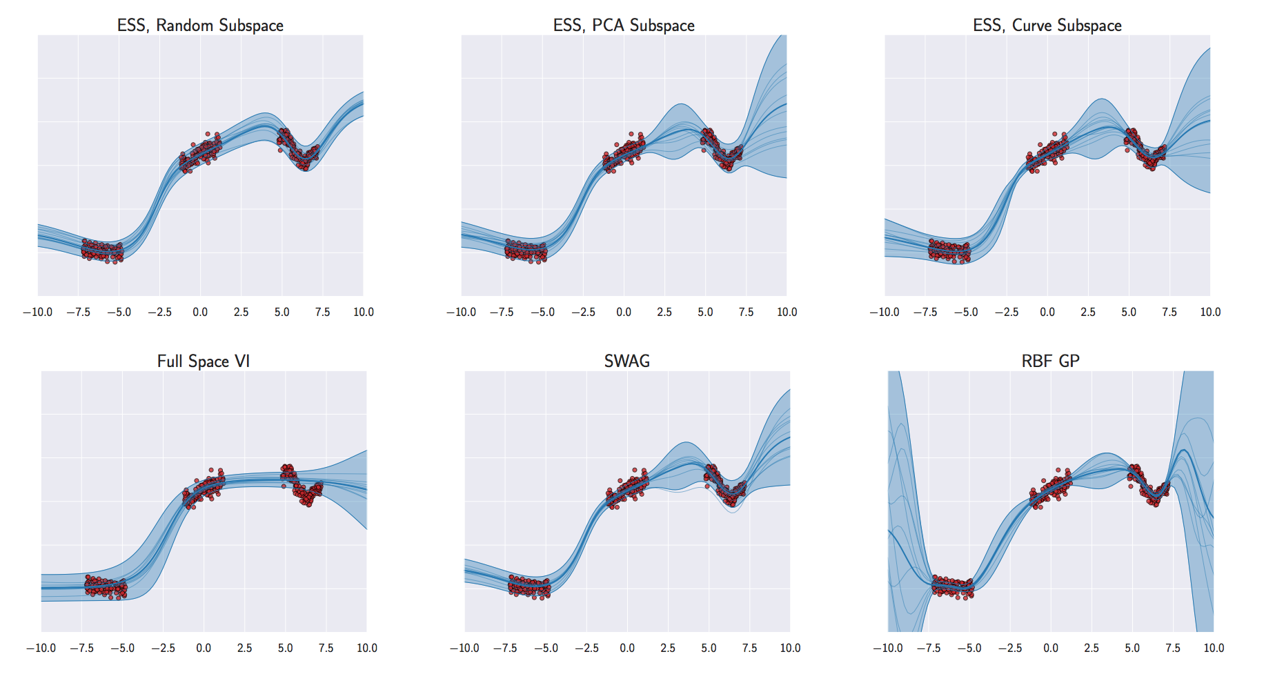
Izmailov et al. (2019)

Deep Gaussian Processes

• Deep architectures allow abstraction of features (Bengio, 2009; Hinton and Osindero, 2006; Salakhutdinov and Murray, n.d.)
• We use variational approach to stack GP models.

Stacked PCA

❮ ❯

Stacked GP

❮ ❯

Analysis of Deep GPs

• Avoiding pathologies in very deep networks Duvenaud et al. (2014) show that the derivative distribution of the process becomes more heavy tailed as number of layers increase.

• How Deep Are Deep Gaussian Processes? Dunlop et al. (n.d.) perform a theoretical analysis possible through conditional Gaussian Markov property.

Stacked GPs (video by David Duvenaud)

Olympic Marathon Data

Gold medal times for Olympic Marathon since 1896. Marathons before 1924 didn’t have a standardised distance. Present results using pace per km. In 1904 Marathon was badly organised leading to very slow times.

Image from Wikimedia Commons http://bit.ly/16kMKHQ

Olympic Marathon Data

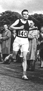
Alan Turing

Probability Winning Olympics?

• He was a formidable Marathon runner.
• In 1946 he ran a time 2 hours 46 minutes.
  • That’s a pace of 3.95 min/km.
• What is the probability he would have won an Olympics if one had been held in 1946?

Olympic Marathon Data GP

Deep GP Fit

• Can a Deep Gaussian process help?

• Deep GP is one GP feeding into another.

Olympic Marathon Data Deep GP

Olympic Marathon Data Deep GP

Olympic Marathon Data Latent 1

Olympic Marathon Data Latent 2

Olympic Marathon Pinball Plot

Della Gatta Gene Data

• Given given expression levels in the form of a time series from Della Gatta et al. (2008).

Della Gatta Gene Data

Gene Expression Example

• Want to detect if a gene is expressed or not, fit a GP to each gene Kalaitzis and Lawrence (2011).

TP53 Gene Data GP

TP53 Gene Data GP

TP53 Gene Data GP

Multiple Optima

Della Gatta Gene Data Deep GP

Della Gatta Gene Data Deep GP

Della Gatta Gene Data Latent 1

Della Gatta Gene Data Latent 2

TP53 Gene Pinball Plot

Step Function Data

Step Function Data GP

Step Function Data Deep GP

Step Function Data Deep GP

Step Function Data Latent 1

Step Function Data Latent 2

Step Function Data Latent 3

Step Function Data Latent 4

Step Function Pinball Plot

Motorcycle Helmet Data

Motorcycle Helmet Data GP

Motorcycle Helmet Data Deep GP

Motorcycle Helmet Data Deep GP

Motorcycle Helmet Data Latent 1

Motorcycle Helmet Data Latent 2

Motorcycle Helmet Pinball Plot

Robot Wireless Ground Truth

Robot WiFi Data

Robot WiFi Data GP

Robot WiFi Data Deep GP

Robot WiFi Data Deep GP

Robot WiFi Data Latent Space

}

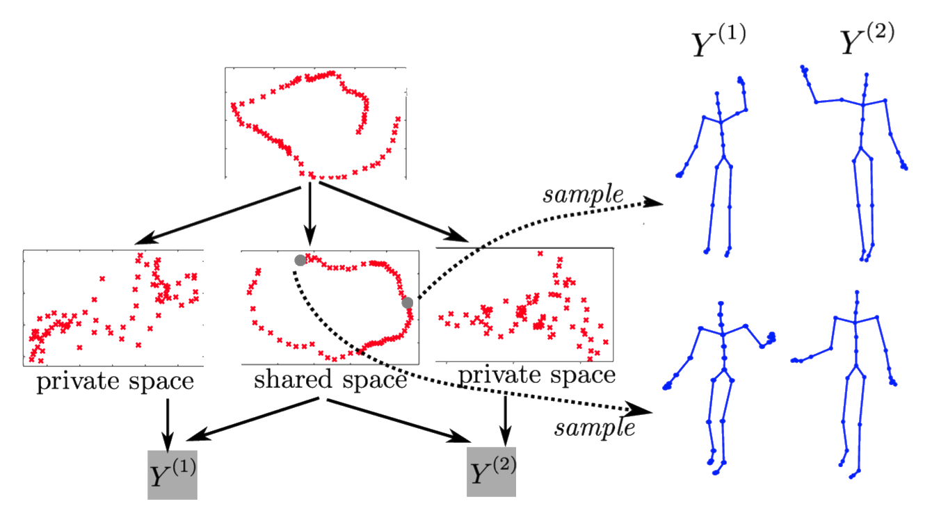
‘High Five’ Motion Capture Data

• ‘High five’ data.
• Model learns structure between two interacting subjects.

Shared LVM

Subsample of the MNIST Data

Fitting a Deep GP to a the MNIST Digits Subsample

Thanks to: Zhenwen Dai and Neil D. Lawrence

Deep Health

References

Álvarez, M.A., Luengo, D., Titsias, M.K., Lawrence, N.D., 2010. Efficient multioutput Gaussian processes through variational inducing kernels, in:. pp. 25–32.
Bengio, Y., 2009. Learning Deep Architectures for AI. Found. Trends Mach. Learn. 2, 1–127. https://doi.org/10.1561/2200000006
Bui, T.D., Yan, J., Turner, R.E., 2017. A unifying framework for Gaussian process pseudo-point approximations using power expectation propagation. Journal of Machine Learning Research 18, 1–72.
Bui, T., Hernandez-Lobato, D., Hernandez-Lobato, J., Li, Y., Turner, R., 2016. Deep Gaussian processes for regression using approximate expectation propagation, in: Balcan, M.F., Weinberger, K.Q. (Eds.), Proceedings of the 33rd International Conference on Machine Learning, Proceedings of Machine Learning Research. PMLR, New York, New York, USA, pp. 1472–1481.
Dai, Z., Damianou, A., Hensman, J., Lawrence, N.D., 2014. Gaussian process models with parallelization and GPU acceleration.
Damianou, A., 2015. Deep Gaussian processes and variational propagation of uncertainty (PhD thesis). University of Sheffield.
Damianou, A., Titsias, M.K., Lawrence, N.D., 2016. Variational inference for latent variables and uncertain inputs in Gaussian processes. Journal of Machine Learning Research 17.
Della Gatta, G., Bansal, M., Ambesi-Impiombato, A., Antonini, D., Missero, C., Bernardo, D. di, 2008. Direct targets of the trp63 transcription factor revealed by a combination of gene expression profiling and reverse engineering. Genome Research 18, 939–948. https://doi.org/10.1101/gr.073601.107
Dunlop, M.M., Girolami, M.A., Stuart, A.M., Teckentrup, A.L., n.d. How deep are deep Gaussian processes? Journal of Machine Learning Research 19, 1–46.
Duvenaud, D., Rippel, O., Adams, R., Ghahramani, Z., 2014. Avoiding pathologies in very deep networks, in:.
Gal, Y., Wilk, M. van der, Rasmussen, C.E., n.d. Distributed variational inference in sparse Gaussian process regression and latent variable models, in:.
Havasi, M., Hernández-Lobato, J.M., Murillo-Fuentes, J.J., 2018. Inference in deep Gaussian processes using stochastic gradient Hamiltonian Monte Carlo, in: Bengio, S., Wallach, H., Larochelle, H., Grauman, K., Cesa-Bianchi, N., Garnett, R. (Eds.), Advances in Neural Information Processing Systems 31. Curran Associates, Inc., pp. 7506–7516.
Hensman, J., Fusi, N., Lawrence, N.D., n.d. Gaussian processes for big data, in:.
Hinton, G.E., Osindero, S., 2006. A fast learning algorithm for deep belief nets. Neural Computation 18, 2006.
Hoffman, M., Blei, D.M., Wang, C., Paisley, J., 2012. Stochastic variational inference, arXiv preprint arXiv:1206.7051.
Izmailov, P., Maddox, W.J., Kirichenko, P., Garipov, T., Vetrov, D.P., Wilson, A.G., 2019. Subspace inference for bayesian deep learning. CoRR abs/1907.07504.
Kalaitzis, A.A., Lawrence, N.D., 2011. A simple approach to ranking differentially expressed gene expression time courses through Gaussian process regression. BMC Bioinformatics 12. https://doi.org/10.1186/1471-2105-12-180
Lawrence, N.D., n.d. Learning for larger datasets with the Gaussian process latent variable model, in:. pp. 243–250.
Lawrence, N.D., Moore, A.J., 2007. Hierarchical Gaussian process latent variable models, in:. pp. 481–488.
MacKay, D.J.C., n.d. Introduction to Gaussian processes, in:. pp. 133–166.
Quiñonero Candela, J., Rasmussen, C.E., 2005. A unifying view of sparse approximate Gaussian process regression. Journal of Machine Learning Research 6, 1939–1959.
Salakhutdinov, R., Murray, I., n.d. On the quantitative analysis of deep belief networks, in:. pp. 872–879.
Salimbeni, H., Deisenroth, M., 2017. Doubly stochastic variational inference for deep Gaussian processes, in: Guyon, I., Luxburg, U.V., Bengio, S., Wallach, H., Fergus, R., Vishwanathan, S., Garnett, R. (Eds.), Advances in Neural Information Processing Systems 30. Curran Associates, Inc., pp. 4591–4602.
Seeger, M.W., Hetzel, A., Dai, Z., Lawrence, N.D., 2017. Auto-differentiating linear algebra. CoRR abs/1710.08717.
Snelson, E., Ghahramani, Z., n.d. Sparse Gaussian processes using pseudo-inputs, in:.
Taigman, Y., Yang, M., Ranzato, M., Wolf, L., 2014. DeepFace: Closing the gap to human-level performance in face verification, in: Proceedings of the IEEE Computer Society Conference on Computer Vision and Pattern Recognition. https://doi.org/10.1109/CVPR.2014.220
Titsias, M.K., n.d. Variational learning of inducing variables in sparse Gaussian processes, in:. pp. 567–574.