AI and Data Science
Systems, Data Science, Biology, Medicine
Autumn Data Science School, Cambridge
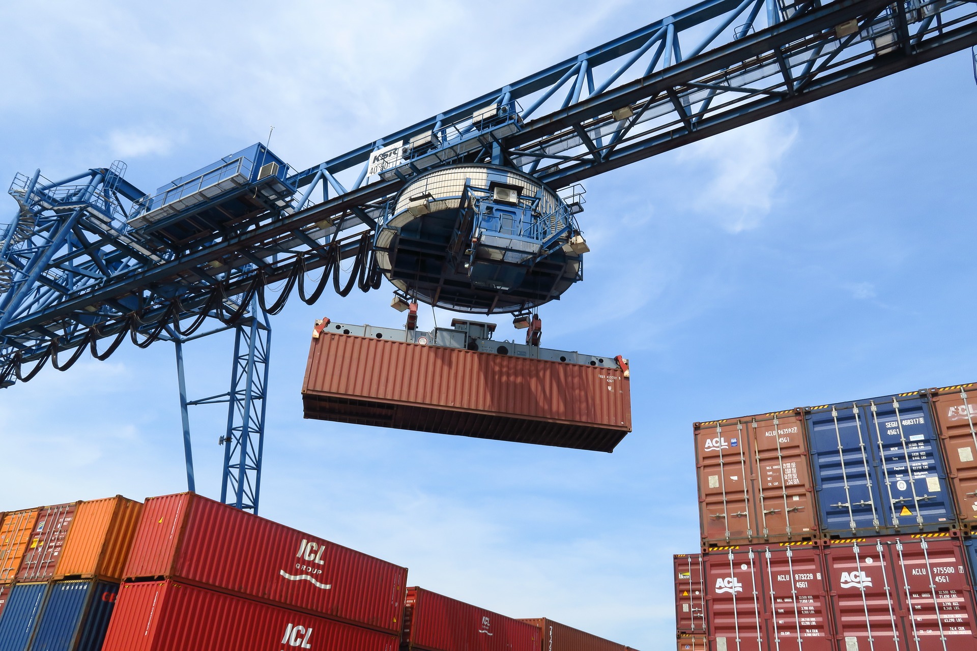
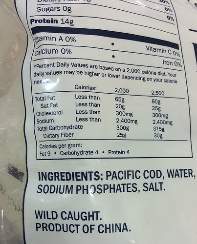
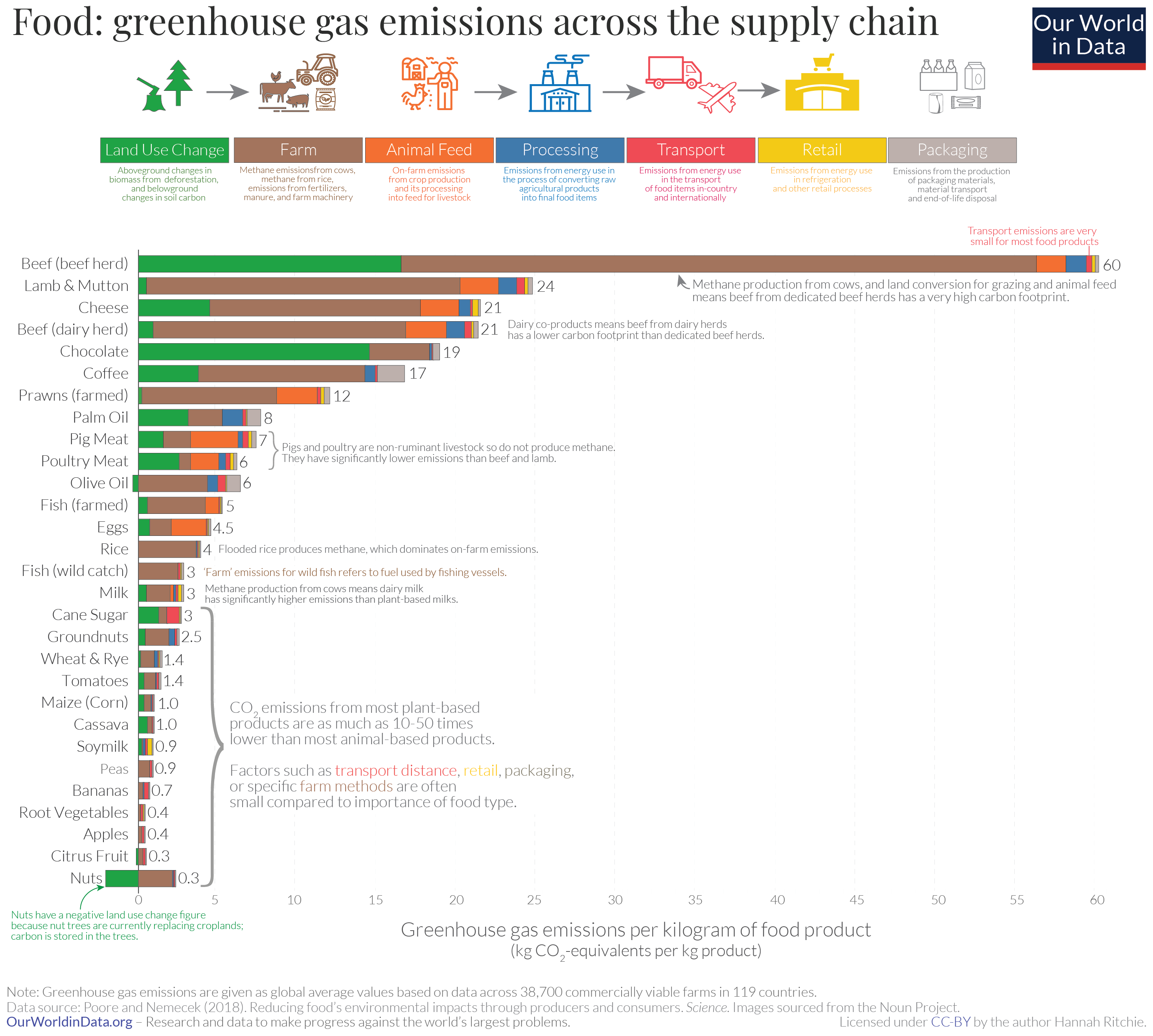
Supply Chain
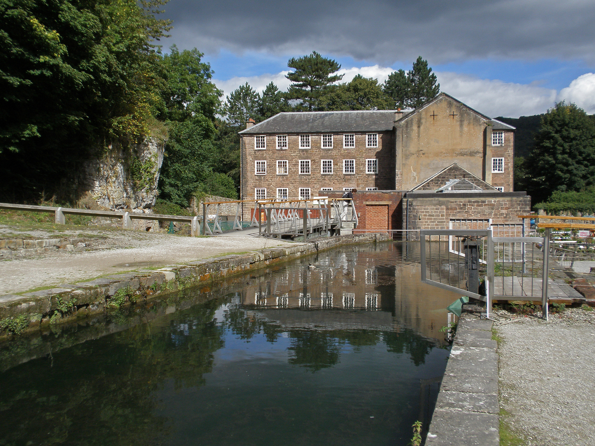
Cromford
Deep Freeze

Deep Freeze
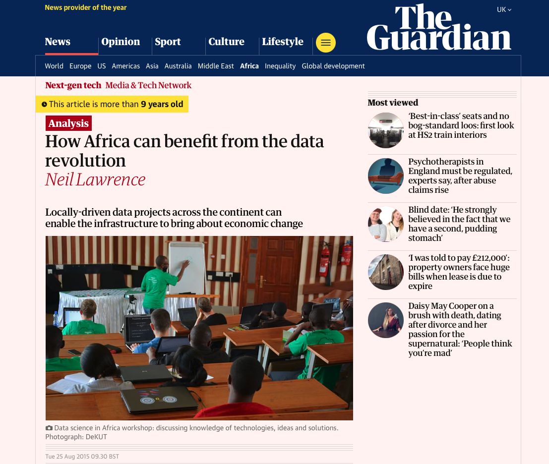
Data Science Africa is a bottom up initiative for capacity building in data science, machine learning and AI on the African continent
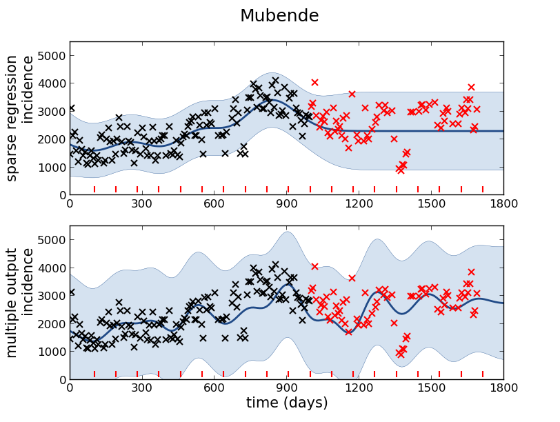
Malaria Prediction in Uganda
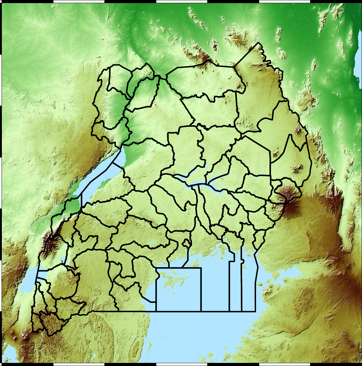
(Andrade-Pacheco
et al., 2014; Mubangizi et al., 2014)
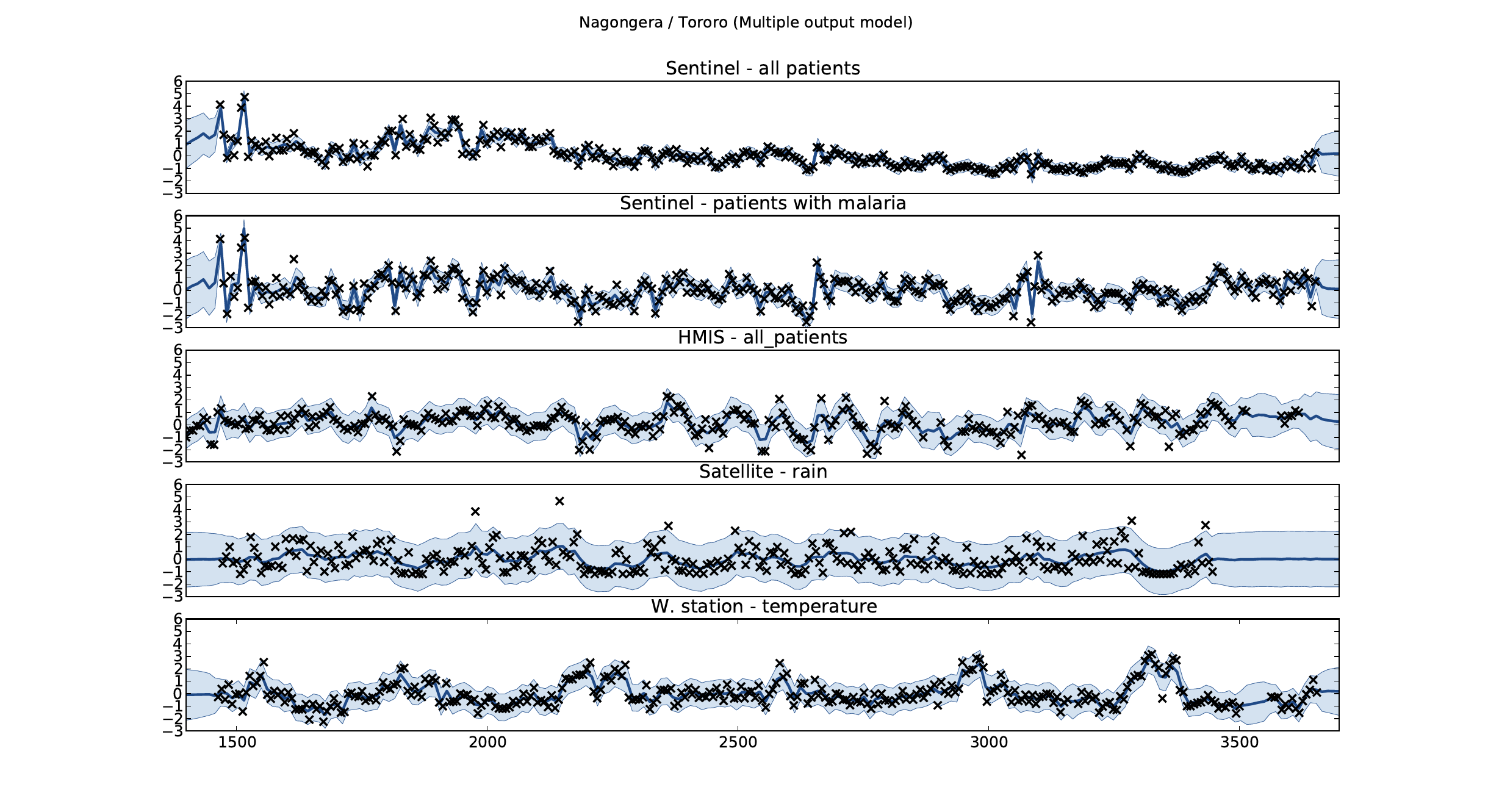
Malaria Prediction in Nagongera (Sentinel Site)
Malaria Prediction in Uganda
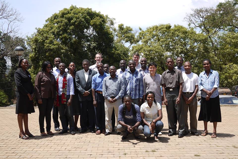
GP School at Makerere
Early Warning System
Early Warning Systems