Jaynes’ World

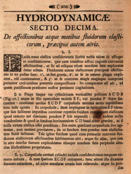
Hydrodynamica

Entropy Billiards

<canvas id="multiball-canvas" width="700" height="500" style="border:1px solid black;display:block;width:100%"></canvas>

<div>Velocity-bin entropy: <output id="multiball-entropy"></output></div>
<div id="multiball-histogram-canvas" style="width:100%;height:250px"></div>

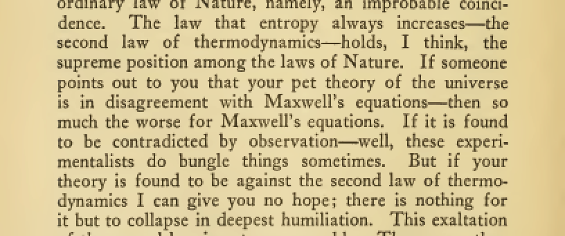
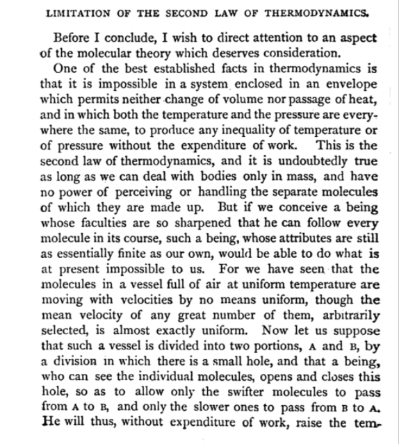
Maxwell’s Demon

Information Theory and Thermodynamics

• Information theory quantifies uncertainty and information
• Core concepts inspired by thermodynamic ideas
• Information entropy \(\leftrightarrow\) Thermodynamic entropy
  • Free energy minimization common in both domains

Entropy

• Entropy \[ S(X) = -\sum_X \rho(X) \log p(X) \]

• In thermodynamics preceded by Boltzmann’s constant, \(k_B\)

Exponential Family

• Exponential family: \[ \rho(Z) = h(Z) \exp\left(\boldsymbol{\theta}^\top T(Z) + A(\boldsymbol{\theta})\right) \]

• Entropy is, \[ S(Z) = A(\boldsymbol{\theta}) - E_\rho\left[\boldsymbol{\theta}^\top T(Z) + \log h(Z)\right] \]

• Where \[ E_\rho\left[T(Z)\right] = \nabla_\boldsymbol{\theta}A(\boldsymbol{\theta}) \] because \(A(\boldsymbol{\theta})\) is log partition function.

• operates as a cummulant generating function for \(\rho(Z)\).

Available Energy

• Available energy: \[ A(\boldsymbol{\theta}) \]
• Internal energy: \[ U(\boldsymbol{\theta}) = A(\boldsymbol{\theta}) + T S(\boldsymbol{\theta}) \]

• Traditional relationship \[ A = U - TS \]
• Legendre transformation of entropy

Work through Measurement

• Split system \(Z\) into two parts:
  • Variables \(X\) - stochastically evolving
  • Memory \(M\) - low entropy partition

Joint Entropy Decomposition

• Joint entropy can be decomposed \[ S(Z) = S(X,M) = S(X|M) + S(M) = S(X) - I(X;M) + S(M) \]

• Mutual information \(I(X;M)\) connects information and energy

Measurement and Available Energy

• Measurement changes system entropy by \(-I(X;M)\)

• Increases available energy

• Difference in available energy: \[ \Delta A = A(X) - A(X|M) = I(X;M) \]

• Can recover \(k_B T \cdot I(X;M)\) in work from the system

Information to Work Conversion

• Maxwell’s demon thought experiment in practice
• Information gain \(I(X;M)\) can be converted to work
• Maximum extractable work: \(W_{max} = k_B T \cdot I(X;M)\)
• Measurement creates a non-equilibrium state
• Information is a physical resource

The Animal Game

• Intelligence as optimal uncertainty reduction
  • 20 Questions game as intuitive example
  • Binary search exemplifies optimal strategy
• Information gain measures question quality
  • Wordle as a more complex example

The 20 Questions Paradigm

Entropy Reduction and Decisions

• Entropy before question: \(S(X)\)
• Entropy after answer: \(S(X|M)\)
• Information gain: \(I(X;M) = S(X) - S(X|M)\)
• Optimal decision maximise \(I(X;M)\) per unit cost

Thermodynamic Parallels

• Intelligence requires work to reduce uncertainty
• Thermodynamic work reduces physical entropy
• Both operate under resource constraints
• Both bound by fundamental efficiency limits

Information Engines: Intelligence as an Energy-Efficiency

• Information can be converted to available energy
• Simple systems that exploit this are “information engines”
• This provides our first model of intelligence

Measurement as a Thermodynamic Process: Information-Modified Second Law

• Measurement is a thermodynamic process
• Maximum extractable work: \(W_\text{ext} \leq -\Delta\mathcal{F} + k_BTI(X;M)\)
• Information acquisition creates work potential

\[ I(X;M) = \sum_{x,m} \rho(x,m) \log \frac{\rho(x,m)}{\rho(x)\rho(m)}, \]

Efficacy of Feedback Control

Channel Coding Perspective on Memory

• Memory acts as an information channel
• Channel capacity limited by memory size: \(C \leq n\) bits
• Relates to Ashby’s Law of Requisite Variety and the information bottleneck

Decomposition into Past and Future

Model Approximations and Thermodynamic Efficiency

• Perfect models require infinite resources
• Intelligence balances measurement against energy efficiency
• Bounded rationality as thermodynamic necessity

Markov Blanket

• Split system into past/present (\(X_0\)) and future (\(X_1\))
• Memory \(M\) creates Markov separation when \(I(X_0;X_1|M) = 0\)
• Efficient memory minimizes information loss

At What Scales Does this Apply?

• Equipartition theorem: \(kT/2\) energy per degree of freedom
• Information storage is a small perturbation in large systems
• Most relevant at microscopic scales

Small-Scale Biochemical Systems and Information Processing

• Microscopic biological systems operate where information matters
• Molecular machines exploit thermal fluctuations
• Information processing enables work extraction

Molecular Machines as Information Engines

• ATP synthase, kinesin, photosynthetic apparatus
• Convert environmental information to useful work
• Example: ATP synthase uses ~3-4 protons per ATP

ATP Synthase: Nature’s Rotary Engine

Jaynes’s Maximum Entropy Principle

• Jaynes (1957): Statistical mechanics as inference with incomplete information

• Maximum entropy principle: most honest description of what we know

• Avoids unwarranted assumptions beyond available data

• Die example: Average result 4.5 instead of 3.5

• Constraints:

  • \(\sum_{n=1}^6 P_n = 1\) (normalization)
  • \(\sum_{n=1}^6 nP_n = 4.5\) (observed average)

The General Maximum-Entropy Formalism

Jaynes’ World

• Zero-player game implementing entropy game
• Distribution \(\rho(Z)\) over state space \(Z\)
• State space partitioned into observables \(X\) and memory \(M\)
• Entropy bounded: \(0 \leq S(Z) \leq N\)

Jaynes’ World

• Unlike animal game (which reduces entropy), Jaynes’ World maximizes entropy

• System evolves by ascending the entropy gradient \(S(Z)\)

• Animal game: max uncertainty → min uncertainty

• Jaynes’ World: min uncertainty → max uncertainty

• Thought experiment: looking backward from any point

• Game appears to come from minimal entropy configuration (“origin”)

• Game appears to move toward maximal entropy configuration (“end”)

\[ \rho(Z) = h(Z) \exp(\boldsymbol{\theta}^\top T(Z) - A(\boldsymbol{\theta})), \] where \(h(Z)\) is the base measure, \(T(Z)\) are sufficient statistics, \(A(\boldsymbol{\theta})\) is the log-partition function, \(\boldsymbol{\theta}\) are the natural parameters of the distribution.}

Exponential Family

• Jaynes showed that entropy optimization leads to exponential family distributions. \[\rho(Z) = h(Z) \exp(\boldsymbol{\theta}^\top T(Z) - A(\boldsymbol{\theta}))\]
• \(h(Z)\): base measure
• \(T(Z)\): sufficient statistics
• \(A(\boldsymbol{\theta})\): log-partition function
• \(\boldsymbol{\theta}\): natural parameters

Information Geometry

• System evolves within information geometry framework
• Entropy gradient \[ \nabla_{\boldsymbol{\theta}}S(Z) = \mathbf{g} = \nabla^2_\boldsymbol{\theta} A(\boldsymbol{\theta}(M)) \]

Fisher Information Matrix

• Fisher information matrix \[ G(\boldsymbol{\theta}) = \nabla^2_{\boldsymbol{\theta}} A(\boldsymbol{\theta}) = \text{Cov}[T(Z)] \]
• Important: We use gradient ascent, not natural gradient

Gradient Ascent

• Gradient step \[ \Delta \boldsymbol{\theta} \propto \mathbf{g} \]
• Natural gradient step \[ \Delta \boldsymbol{\theta} \propto \eta G(\boldsymbol{\theta})^{-1} \mathbf{g} \]

System Evolution

Start State

• Low entropy, near lower bound
• Highly structured information in \(M\)
• Strong temporal dependencies (high non-Markovian component)
• Precise values for \(\boldsymbol{\theta}\) uncertainty in other parameter characteristics
• Uncertainty principle balances precision vs. capacity

End State

• Maximum entropy, approaching upper bound \(N\)
• Zeno’s paradox: \(\nabla_{\boldsymbol{\theta}}S \approx 0\)
• Primarily Markovian dynamics
• Steady state with no further entropy increase possible

Key Point

• Both minimal and maximal entropy distributions belong to exponential family
• This is a direct consequence of Jaynes’ entropy optimization principle
• System evolves by gradient ascent in natural parameters
• Uncertainty principle governs the balance between precision and capacity

Jaynes’ World

• Configuration is primary; parameters emerge from monitoring choices
• Distribution captures uncertainty about possible configurations
• Framework for observer-free dynamics and entropy-based emergence

Fundamental Structure: Configuration and Uncertainty

Configuration as Primary Reality

• Configuration: actual structural relationships between variables
• Primary ontological reality, independent of observation
• Parameters and mathematics are epistemic tools for tracking configuration

Uncertainty Distribution Over Configurations

• Density matrix \(\rho\): uncertainty about which configuration is actual
• Not the configuration itself, but probability over possible configurations
• Von Neumann entropy: amount of uncertainty/disorder in our knowledge

Emergence of Mathematical Structure

Exponential Family as Inevitable Consequence

• Exponential family form emerges automatically
• Result of minimizing uncertainty subject to resolution constraints
• Natural parameters \(\theta_i\) are Lagrange multipliers from optimization

System Structure Through Uncertainty Dynamics

• Full set of variables: \(Z = \{Z_1, Z_2, \dots, Z_n\}\)
• Partition emerges from uncertainty resolution:
  • Active variables \(X(\tau)\): resolvable above threshold \(\varepsilon\)
  • Latent variables \(M(\tau)\): uncertainty reservoir below threshold

.

Derived Mathematical Objects

• Log-partition function: \(A(\boldsymbol{\theta}) = \log Z(\boldsymbol{\theta})\)
• Von Neumann entropy: \(S(\boldsymbol{\theta}) = A(\boldsymbol{\theta}) - \boldsymbol{\theta}^\top \nabla A(\boldsymbol{\theta})\)
• Fisher Information: \(G_{ij}(\boldsymbol{\theta}) = \frac{\partial^2 A}{\partial \theta_i \partial \theta_j}\)
• All emerge from uncertainty minimization, not imposed assumptions

Resolution Constraints and Discrete Structure

• Maximum uncertainty capacity: \(N\) bits
• Minimum detectable resolution: \(\varepsilon\)
  
• Discrete transitions emerge from continuous underlying uncertainty

Uncertainty-Driven Dynamics

Core Principle: Uncertainty Resolution

• System evolves to resolve uncertainty about configuration
• Steepest ascent in entropy = fastest uncertainty resolution \[ \frac{\text{d}\boldsymbol{\theta}}{\text{d}\tau} = -G(\boldsymbol{\theta}) \boldsymbol{\theta} \]
• Parameters track this uncertainty resolution process

Variable Activation Through Uncertainty Thresholds

• Active variables: \(X(\tau) = \left\{ i \mid \left| \frac{\text{d}\theta_i}{\text{d}\tau} \right| \geq \varepsilon \right\}\)
• Activation occurs when uncertainty gradients exceed resolution threshold
• Configuration changes manifest as parameter threshold crossings

Information Geometry of Uncertainty Evolution

• Fisher matrix partitioning reflects uncertainty structure
• \(G_{XX}\): resolvable uncertainty geometry
  
• \(G_{MM}\): latent uncertainty reservoir
• \(G_{XM}\): coupling between resolved and unresolved uncertainty

Lemma 1: Form of the Minimal Entropy Configuration

• Minimal entropy state: \(\rho(\boldsymbol{\theta}_o) = \frac{1}{Z(\boldsymbol{\theta}_o)} \exp\left( \sum_i \theta_{oi} H_i \right)\)
• All parameters sub-threshold: \(|\dot{\theta}_{oi}| < \varepsilon\)
• Regular, continuous, and detectable above resolution scale

Lemma 2: Symmetry Breaking

• If \(\theta_k \in M(\tau)\) and \(|\dot{\theta}_k| \geq \varepsilon\), then \(\theta_k \in X(\tau + \delta)\)
• Latent variables can become active when their rate of change exceeds threshold
• Mechanism for emergence of new active variables

Perceived Time

• Entropy-time: \(t(\tau) := S_{X(\tau)}(\tau)\)
• Measures accumulated entropy of active variables

Monotonicity of Perceived Time

• \(t(\tau_2) \geq t(\tau_1)\) for all \(\tau_2 > \tau_1\)
• Perceived time always increases
• Implies irreversibility of the system

Corollary: Irreversibility

• \(t(\tau)\) increases monotonically
• Prevents time-reversal globally
• Provides an arrow of time for the system

2. In regions where parameters are weakly coupled to entropy change (low \(\boldsymbol{\theta}^\top \nabla_\boldsymbol{\theta} S[\rho_\boldsymbol{\theta}]\)), perceived time flows slowly.

3. At critical points where parameters become orthogonal to the entropy gradient (\(\boldsymbol{\theta}^\top \nabla_\boldsymbol{\theta} S[\rho_\boldsymbol{\theta}] \approx 0\)), the time parameterization approaches singularity indicating phase transitions in the system’s information structure. }

Conjecture: Frieden-Analogous Extremal Flow

• When latent-to-active flow is extremal, system exhibits critical slowing
• System entropy separates into active variables \(I = S[\rho_X]\) and “intrinsic information” \(J = S[\rho_{X|M}]\)
• Analogous to Frieden (1998) extreme physical information principle \(\delta(I - J) = 0\)

From Maximum to Minimal Entropy

• Maximum entropy = minimum assumptions
• Minimal entropy = maximum structure/information
• Same mathematical framework, different constraints

Minimal Entropy States in Quantum Systems

Histogram Game

Two-Bin Histogram Example

• Simplest example: Two-bin system
• States represented by probability \(p\) (with \(1-p\) in second bin)

Entropy

• Entropy \[ S(p) = -p\log p - (1-p)\log(1-p) \]
• Maximum entropy at \(p = 0.5\)
• Minimal entropy at \(p = 0\) or \(p = 1\)

Natural Gradients vs Steepest Ascent

\[ \Delta \theta_{\text{steepest}} = \eta \frac{\text{d}S}{\text{d}\theta} = \eta p(1-p)(\log(1-p) - \log p). \] \[ G(\theta) = p(1-p) \] \[ \Delta \theta_{\text{natural}} = \eta(\log(1-p) - \log p) \]

Gradient Ascent in Natural Parameter Space

Gradient Ascent Evolution

Entropy Evolution

Trajectory in Natural Parameter Space

Uncertainty Principle

• Information reservoir variables (\(M\)) map to natural parameters \(\boldsymbol{\theta}(M)\)
• Challenge: Need both precision in parameters and capacity for information

Formal Derivation of the Uncertainty Principle

• Information-theoretic derivation
• Begins with Shannon entropy constraints
• Reaches uncertainty bound through variational analysis

Definition of Capacity Variables

• Capacity variables \(c(M)\) precisely defined:
  • Measure information storage potential
  • Fourier-conjugate to parameters

Capacity \(\leftrightarrow\) Precision Paradox

• Fundamental trade-off emerges:
• \(\Delta\boldsymbol{\theta}(M) \cdot \Delta c(M) \geq k\)
• Cannot simultaneously have perfect precision and maximum capacity

Quantum vs Classical Information Reservoirs

• Near origin: quantum-like
  • Wave encoding of capacity, non-local correlations
  • Uncertainty principle saturated
• Higher entropy: Transition to “classical” behavior
  • From wave-like to particle-like information storage
  • Local rather than distributed encoding

Quantitative Demonstration

• Numerical example showing uncertainty principle
• Demonstrates trade-off across parameter space
• Shows saturation at minimal entropy

Maximum Entropy and Density Matrices

• Jaynes recognized density matrices as quantum extension
• Same maximum entropy principle applies
• Von Neumann entropy: \(S = -\text{Tr}(\rho \log \rho)\)
• Provides unified approach to classical and quantum systems

Quantum States and Exponential Families

• Minimal entropy quantum states belong to exponential families
• Classical: \(f(x; \theta) = h(x) \cdot \exp[\eta(\theta)^\top \cdot T(x) - A(\theta)]\)
• Density matrix: \(\rho = \exp(-\mathbf{R}^T \cdot \mathbf{G} \cdot \mathbf{R} - Z)\)

Fisher Information and the Uncertainty Principle

• Matrix G relates to quantum Fisher information: \[ \mathbf{G} = \text{QFIM}/4 \]
• Uncertainty-information relationship: \[ V \cdot \text{QFIM} \geq \frac{\hbar^2}{4} \]

Connection to Information Engines

• Minimal entropy states are optimal information engines
• They achieve maximum precision allowed by quantum mechanics
• Examples: squeezed states, coherent states, Gaussian entangled states

Minimal Entropy States

• Minimal entropy states (“origin” in Jaynes’ World)
• Constrained by uncertainty principle:
  • \(\Delta\boldsymbol{\theta}(M) \cdot \Delta c(M) \geq k\)
• Fundamental limit on information structure

Structure of Minimal Entropy States

• Minimal entropy states have:
  • Pure Gaussian form in parameter space
  • Exactly saturate uncertainty bound
  • Belong to exponential family
• Total entropy bounded: \(S(Z) = 0\) for minimal states, with \(0 \leq S(Z) \leq N\) overall

Fisher Information and Minimal Uncertainty

• Precision matrix \(\boldsymbol{\Lambda}\) directly related to Fisher information
• \(\mathbf{G} = \boldsymbol{\Lambda}/2\) (Fisher information matrix)
• Creates relationship:
  • \(\mathbf{V} \cdot \mathbf{G} \geq k^2\)

Connection to Information Reservoirs

• Information reservoir \(M\) at minimal entropy:
  • Stores information in wave-like patterns
  • Distributes uncertainty optimally
  • Creates non-local correlations

Implications for System Evolution

• As system evolves from minimal entropy:
  • Uncertainty bound becomes less saturated
  • Information encoding transitions from wave-like to particle-like
  • System moves from quantum-like to classical-like behavior

Physical Interpretation

• Minimal entropy states analogous to:
  • Squeezed states in quantum optics
  • Ground states of many-body systems
  • Coherent structures in complex systems
• Quantum states have minimum entropy due to uncertainty principle
• Minimal entropy states are pure Gaussian states
• These represent fundamental information engines

Von Neumann Entropy

• Quantum analog of Shannon entropy: \[S(\rho) = -\text{Tr}(\rho \ln \rho)\]
• Pure states: \(S(\rho) = 0\)
• Mixed states: \(S(\rho) > 0\)

Quantum Uncertainty Principle as a Constraint

• Position-momentum uncertainty: \[\Delta x \cdot \Delta p \geq \frac{\hbar}{2}\]
• Matrix form for multiple variables: \[V + i\frac{\hbar}{2}\Omega \geq 0\]

Density Matrices and Exponential Families

• Minimal entropy quantum states belong to exponential families
• Classical: \(f(x; \theta) = h(x) \cdot \exp[\eta(\theta)^\top \cdot T(x) - A(\theta)]\)
• Density matrix: \(\rho = \exp(-\mathbf{R}^T \cdot \mathbf{G} \cdot \mathbf{R} - Z)\)

Classical Exponential Family

Quantum Minimal Entropy State

Gradient Ascent and Uncertainty Principles

• Gradient ascent on entropy naturally respects uncertainty principles
• Systems evolve from quantum-like to classical-like regimes
• Uncertainty ellipses visualize this transition

Gaussian Systems and Uncertainty

• Multivariate Gaussian: \(\rho(z) \propto \exp\left(-\frac{1}{2}z^T \Lambda z\right)\)
• Precision matrix \(\Lambda\) determines uncertainty structure
• Entropy: \(S = \frac{1}{2}\log\det(V) + \text{constant}\)
• Uncertainty principle: \(\Delta x \cdot \Delta p \geq \frac{\hbar}{2}\)

Multivariate Systems and Saddle Points

• Multiple position-momentum pairs create rich dynamics
• System naturally slows near saddle points
• Some variables remain quantum-like while others become classical-like

Eigenvalue Evolution

Uncertainty Products Evolution

Entropy Evolution During Gradient Ascent

Evolution of Uncertainty Products

Visualising the Parameter-Capacity Uncertainty Principle

• Uncertainty principle: \(\Delta\theta \cdot \Delta c \geq k\)
• Minimal uncertainty states form ellipses in phase space
• Quantum-like properties emerge from information constraints
• Different uncertainty states visualized as probability distributions

Visualisation of the Uncertainty Principle

Scaling to Large Systems: Emergent Statistical Behavior

• Scale to systems with 1000+ position-momentum pairs
• Observe emergent statistical behaviors
• Identify clusters of similar dynamical patterns
• Analyze quantum-classical phase transitions

Emergent Statistical Behaviors

• Statistical phase transitions emerge
• Natural clustering of dynamical behaviors
• Scale-invariant patterns across system sizes
• Quantum-classical boundary becomes a statistical property

Large-Scale Gradient Ascent

Four-Bin Saddle Point Example

• Four-bin system creates 3D parameter space
• Saddle points appear where:
  • Gradient is zero
  • Some directions increase entropy
  • Other directions decrease entropy
• Information reservoirs form in critically slowed directions

Saddle Point Example

Entropy Evolution

Saddle Points

Saddle Point Seeking Behaviour

Dynamical System

Entropy Bounds and Compactness

Resolution Constraints

Relationship Between Resolution Threshold and Entropy Bound

Multi-Scale Dynamics and Observable Separation

Observable Partitioning

Schur Complement Analysis

Sparsification Through Entropy Maximization

Action Functional Representation

Computational Implications

Emergence of Time

Information Geometry and Resolution Constraints

Information-Theoretic Interpretation

Entropy Maximization

Information Flow and Topography

Resolution and Uncertainty

Temporal Information Dynamics

Connections to Physical Theories

Frieden’s Extreme Physical Information

Conclusion

Spontaneous Organization Through Entropy Maximization

• Can entropy maximization lead to information organization
• Requires: mutual information increases despite overall entropy growth
• Would provides theoretical foundation for emergence of structure
• Needs notion of locality or topology to be fully meaningful

Formal Analysis of Spontaneous Organization

• Joint entropy decomposition: \(S[p(z,t)] = S(X) + S(M) - I(X;M)\)
• Turns derivative: \(\frac{\text{d}S}{\text{d}t} = \frac{\text{d}S(X)}{\text{d}t} + \frac{\text{d}S(M)}{\text{d}t} - \frac{\text{d}I(X;M)}{\text{d}t}\)
• Spontaneous organization when: \(\frac{\text{d}I(X;M)}{\text{d}t} > 0\)

Fisher Information and Multiple Timescales in Spontaneous Organization

Multiple Timescales and Mutual Information Growth

• Fisher information: \(G_{ij}(\boldsymbol{\theta}) = \mathbb{E}\left[\frac{\partial \log p(z|\boldsymbol{\theta})}{\partial \theta_i}\frac{\partial \log p(z|\boldsymbol{\theta})}{\partial \theta_j}\right]\)
• Multiple timescales: \(\eta_X \gg \eta_M\)
• Spontaneous organization requires: \(\|\nabla_{\boldsymbol{\theta}_X}S(X)\|^2 > \|\nabla_{\boldsymbol{\theta}_X}S\|^2\)

Condition for Information Structure Emergence

• Mutual information gradient: \(\nabla_{\boldsymbol{\theta}_X}I(X;M) \approx \nabla_{\boldsymbol{\theta}_X}S(X) - \nabla_{\boldsymbol{\theta}_X}S\)
• Organization emerges when entropy gradients diverge in direction
• Fast variables \(X\) explore state space while slow variables \(M\) capture persistent patterns

Adiabatic Elimination and Effective Dynamics

• Adiabatic elimination: fast variables reach quasi-equilibrium for each slow configuration
• Condition: \(\frac{\text{d}I(X;M)}{\text{d}t} \approx -\eta_M \text{tr}(\mathbf{H}_{XM})\)
• Organization occurs when \(\text{tr}(\mathbf{H}_{XM}) < 0\)
• System develops correlations that maximize entropy efficiently

Locality Through Conditional Independence

• Few slow modes can induce conditional independence
• Creates effective locality and modularity
• Emerges naturally from eigenvalue structure

Entropy Decomposition with Conditional Mutual Information

• Joint entropy decomposition with subsets of X: \(X = \{X^1, X^2, ..., X^K\}\)
• \(S(X, M) = S(M) + \sum_{k=1}^K S(X^k|M) - \sum_{k=1}^K \sum_{j<k} I(X^k; X^j|M)\)
• Conditional mutual information \(I(X^k; X^j|M)\) measures remaining dependencies

Conditional Independence and Locality

• For Gaussian systems, conditional independence requires block-diagonal precision matrix \(\Lambda_{X|M}\)
• Off-diagonal blocks → conditional mutual information \(I(X^k; X^j|M)\)
• Eigenvalue separation determines how effectively slow modes absorb dependencies
• Larger gaps → better factorization → stronger locality

Connection to Eigenvalue Structure

• Few small eigenvalues → strong conditional independence
• Eigenvectors of these slow modes define “information pathways”
• Creates natural graph structure of dependencies
• Analogous to order parameters in physical systems

Conditional Independence Visualization

Dependency Network Structure

Information Topography

• Information topography: landscape of information flow
• “Distance” between variables: \(d_I(X^i, X^j) = \frac{1}{I(X^i; X^j|M) + \epsilon}\)
• Creates intuitive notions of “information watersheds” and “channels”

Properties of Information Topography

• Non-Euclidean, dynamic, and hierarchical
• Shaped by eigenvalue spectrum separation
• Quantifies “information distance” and “barriers”
• Provides unified view of modularity across systems

Information Topography Visualization

Information Topography Eigenspectrum

3D Information Landscape

Temporal Markovian Decomposition

• \(X\) divided into past/present \(X_0\) and future \(X_1\)

• Same slow modes that induce spatial modularity also mediate temporal dependencies

• Conditional mutual information: \[ I(X_0; X_1 | M) = \sum_{x_0,x_1,m} p(x_0,x_1,m) \log \frac{p(x_0,x_1|m)}{p(x_0|m)p(x_1|m)} \]

• Measures dependency between past and future given memory state

• Perfect Markovianity: \(I(X_0; X_1 | M) = 0\)

• Slow modes serve dual purpose:

  1. Creating spatial modularity through conditional independence
  2. Providing temporal memory that bridges past and future

• Eigenvalue spectrum determines both spatial and temporal structure

• Fundamental tension between:

  • Minimal entropy in slow modes (efficiency)
  • Spatial conditional independence (modularity)
  • Temporal conditional independence (memory)

• Creates uncertainty principle with necessary trade-offs

Emergence of Conditional Independence Through Entropy Maximization

• Can conditional independence structures emerge naturally?
• Use gradient ascent on entropy to see eigenvalue structures form
• Observe how slow modes naturally acquire cross-system dependencies
• Track the emergence of conditional independence

Emergent Conditional Independence

• Natural eigenvalue separation into slow and fast modes
• Strong cross-system dependencies become conditionally independent
• Block structure emerges in conditional mutual information matrix
• Locality through conditional independence arises naturally

Fundamental Tradeoffs in Information Processing Systems

• Three fundamental properties with mathematical formulations:

  • Information Capacity: Variances of slow modes \(\sigma_i^2 \propto \frac{1}{\lambda_i}\)
  • Modularity: Conditional independence \(I(X^i; X^j | M) \approx 0\) between modules
  • Memory: Markovian dynamics \(I(X_0; X_1 | M) = 0\) for temporal information

• Mathematical uncertainty relation: \(\mathcal{C}(M) \cdot \mathcal{S}(X|M) \cdot \mathcal{T}(X_0, X_1|M) \geq k\)

• Rigorous mathematical definitions:

  • \(\mathcal{C}(M) = \sum_{i=1}^{d_M} \frac{1}{\lambda_i} = \sum_{i=1}^{d_M} \sigma_i^2\) (Information capacity)
  • \(\mathcal{S}(X|M) = \sum_{i \neq j} I(X^i; X^j | M)\) (Modularity)
  • \(\mathcal{T}(X_0, X_1|M) = I(X_0; X_1 | M)\) (Memory)

• Imposes fundamental limits on simultaneous optimization

• Markov property emerges when slow modes capture all temporal dependencies

• Mathematical tradeoffs between properties:

  • Enhanced memory requires higher capacity slow modes (\(\uparrow \mathcal{C}(M)\))
  • Stronger modularity constrains information flow paths (\(\downarrow \mathcal{S}(X|M)\))
  • Higher information capacity may require more physical resources

The Duality Between Modularity and Memory

• Modularity and memory as dual aspects of the same phenomena:
  • Modularity = “Spatial memory” (independence across space given M)
  • Memory = “Temporal modularity” (independence across time given M)
• Both rely on conditional independence mediated by slow modes
• Same eigenvalue structure determines both properties
• Explains why highly modular systems often have sophisticated memory

Is Landauer’s Limit Related to Shannon’s Gaussian Channel Capacity?

• Memory \(\equiv\) Communication through time

• Storage is transmission to future

• Both limited by thermal noise

• At Landauer’s limit: \(E = k_BT\)

• Gives \(\frac{S}{N} = 1\)

• Results in capacity of \(\frac{1}{2}\) bit/s

• Fundamental connection between energy and information

Implications for Information Engines

• Information engines must overcome thermal noise
• Related threshold for:
  • Information erasure
  • Information transmission
• Temperature sets fundamental noise floor

Detecting Transitions with Moment Generating Functions

• MGF: \(M_Z(t) = \mathbb{E}[e^{tZ}] = \exp(A(\theta+t) - A(\theta))\)
• Cumulant generating function: \(K_Z(t) = \log M_Z(t)\)
• Quantum-like variables: Oscillatory MGF behavior
• Classical variables: Monotonic MGF growth
• MGF reveals channel properties without needing state information

Information Reservoirs

Classical Hierarchical Memory Structure

\[ p(X|M) \approx \prod_i p(X_i|M_{\text{pa}(i)}) \]

Variable Transitions

\[ M_Z(t) = E[e^{t \cdot Z}] = \exp(A(\boldsymbol{\theta}+t) - A(\boldsymbol{\theta})). \]

\[ K_Z(t) = \log M_Z(t) = A(\boldsymbol{\theta}+t) - A(\boldsymbol{\theta}). \]

\[ \frac{d^2}{dt_i^2}K_Z(t)|_{t=0} = \frac{\partial^2 A(\boldsymbol{\theta})}{\partial \theta_i^2}. \]

Hierarchical Memory Organization Example

• Classical information reservoirs organize hierarchically
• Variables separate into distinct timescale bands
• Fast variables: rapidly changing, high processing capacity
• Slow variables: gradually changing, high memory capacity
• Connect across scales for efficient information processing

Conceptual Framework

Conclusion

Unifying Perspectives on Intelligence

• Intelligence through multiple lenses:
  • Entropy game: Intelligence as optimal questioning
  • Information engines: Intelligence as energy-efficient computation
  • Least action: Intelligence as path optimization
  • Schrödinger’s bridge: Intelligence as probability transport
• Jaynes’ world: Initial attempt to Bridge between different views.

A Unified View of Intelligence Through Information

• Converging perspectives on intelligence:

  • Efficient entropy reduction (Entropy Game)
  • Energy-efficient information processing (Information Engines)
  • Path optimization in information space (Least Action)
  • Optimal probability transport (Schrödinger’s Bridge)

• Unified core: Intelligence as optimal information processing

• Implications:

  • Fundamental limits on intelligence
  • New metrics for AI systems
  • Principled approach to cognitive modeling
  • Information-theoretic approaches to learning

Research Directions

• Open questions:
  • Information-theoretic intelligence metrics
  • Physical limits of intelligent systems
  • Connections to quantum information theory
  • Practical algorithms based on these principles
  • Biological implementations of information engines
• Applications:
  • Active learning systems
  • Energy-efficient AI
  • Robust decision-making under uncertainty
  • Cognitive architectures