Information, Energy and Intelligence
What Emerges from Internal Adjudicability?
Cambridge Philosophical Society - David MacKay Memorial Meeting, Cambridge University Engineering Department
In Memory of David MacKay
David MacKay (1967-2016)
- Information theory and inference
- Neural networks and learning algorithms
- Sustainable energy and physical limits
Cut through hype with careful reasoning
How many Lightbulbs?
This Talk
David’s Approach:
- Start with fundamental principles
- Build rigorous mathematical framework
- Apply to real systems
- Use numbers to test claims
Ultimate

Games
- David was a playful person.
- Physics puzzles
- Ultimate Frisbee.
- Ultimate “spirit of the game”
- Ultimiate is a self-adjudicating game
The Munchkin Provision

Munchkin Card Game
Rules may be inconsistent … so …
Any other disputes should be settled by loud arguments, with the owner of the game having the last word.
Munckin Rules (Jackson, 2001)
A Tautology
Self-governing systems cannot refer to external arbitration.
Information
Information and Entropy
- Probability and information theory …
- David’s group meetings from February 1998.
- MN codes, fountain codes, turbocodes
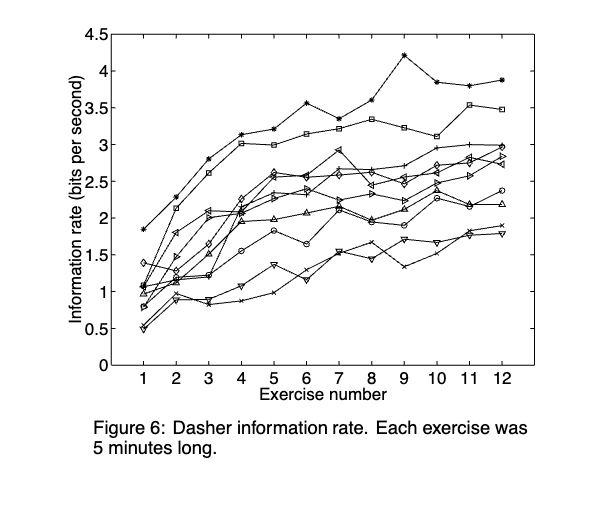
Dasher
Ward et al. (2000)
Dasher
Dasher
Thermalisation from Different Initial Conditions
- 9 balls on a \(3 \times 3\) grid;
- Different starting conditions.
Initialisation: Display:
Sampling Two Dimensional Variables
Correlation
- Correlation is when two variables are dependent
Sampling Two Dimensional Variables
Jaynes and Maximum Entropy

Maximum Entropy Motivation
- Jaynes (1957): Statistical mechanics as inference with incomplete information
- Maximum entropy principle: maximise uncertainty given constraints
- Avoids unwarranted assumptions beyond available data
Dice Example
- Dice example: Average result 4.5 instead of 3.5
- Constraints:
- \(\sum_{n=1}^6 P_n = 1\) (normalization)
- \(\sum_{n=1}^6 nP_n = 4.5\) (observed average)
Die Roll Simulation
Rolls: 0
Sample mean: —
H(p): —
Outcome weights (auto-normalised to probabilities)
The General Maximum-Entropy Formalism
\[ p_i = \frac{\exp(-\lambda_1 f_1(x_i) - \ldots - \lambda_m f_m(x_i))}{Z(\lambda_1,\ldots,\lambda_m)} \] \[ Z(\ldots) = \sum_{i=1}^n \exp(-\lambda_1 f_1(x_i) - \ldots - \lambda_m f_m(x_i)) \] \[ \langle f_k \rangle = -\frac{\partial}{\partial \lambda_k}\log Z(\lambda_1,\ldots,\lambda_m) \quad k=1,2,\ldots,m. \]
Exponential Family
\[ p(X|\boldsymbol{\theta}) = \exp\left(\sum_i \theta_i T(X) - \phi(\boldsymbol{\theta})\right) \] where \(\theta_i = -\lambda_i\)
Waterhouse, MacKay and Robinson
From Waterhouse et al. (n.d.)
Independent Gaussians
Correlated Gaussians
Anticorrelated Gaussians
The Classical Observer
The Classical Observer - Correlated
The Classical Observer - Anti-correlated
Back to self adjudication
The No-Barber Principle
Russell’s Barber Paradox:
Barber shaves all who don’t shave themselves
Does the barber shave themselves?
Paradox: Definition includes itself in scope
No External Adjudicators
Forbidden:
- External observer
- Pre-specified outcome space
- Privileged decomposition
- External time parameter
No appeal to structure outside the game
The Game
The Classical Observer - Inaccessible
Entropy and Impossibility
- We don’t see see the outcome space
- But we summarise it using entropy
- Entropy gives a single number measuring uncertainty
Entropy and Impossibility
- Each distribution gets a score \(\rightarrow\) compare them
- Induces ordering from low to high uncertainty
- Formally: a functor from FinProb to \((\Re, \leq)\)
Marginal and Joint
- Marginal entropy of variable \(i\): \(h_i\)
- Joint entropy of system: \(H\)
- Multiinformation \(I = \sum_i h_i - H\)
Energy
Energy Constraints
- Normally we derive physical laws by
Maximise entropy subject to energy conservation
The Conservation Law
Marginal Entropy Conservation
\[ \sum_{i=1}^N h_i = C \]
Entropy Constraints
- Now derive game rules by
Maximise joint entropy subject to marginal entropy conservation
The \(I + H = C\) Structure
\[ \sum_{i=1}^N h_i = C \]
What does this conservation imply for dynamics?
Multi-Information: Measuring Correlation
\[ I = \sum_{i=1}^N h_i - H \]
- \(I = 0\): Independent variables
- \(I > 0\): Correlated variables
- Larger \(I\) = more correlation
Measures “shared information”
‘Information Action’
\[ I + H = C \]
Conserved quantity splits into two parts
Analogy to classical mechanics:
- Energy: \(T + V = E\)
- Information: \(I + H = C\)
Physical Analogy
| Classical Mechanics | Information System |
|---|---|
| Kinetic energy \(T\) | Joint entropy \(H\) |
| Potential energy \(V\) | Multi-information \(I\) |
| Conservation: \(T + V = E\) | Conservation: \(H + I = C\) |
System “rolls downhill” from correlation to entropy
Information Relaxation
- Second law: Entropy increases (\(\dot{H} > 0\))
- Conservation: \(I + H = C\) (constant)
- Therefore: Correlation decreases (\(\dot{I} < 0\))
Physical intuition
- Compressed spring \(\rightarrow\) released energy
- Correlated variables \(\rightarrow\) independent variables
- Potential \(\rightarrow\) kinetic
Visualisation: Relaxation Dynamics
Information Relaxation Dynamics
Long Story Short
- Can derive GENERIC-like dynamics.
- Origin suggests von Neumann entropy more natural than Shannon.
Connections
- Nice connections between.
- Thermodynamics and Inference (Jaynes).
- Information Geometry and GENERIC.
- Inaccessibility and noncommutative probability.
Energy
MacKay (2008)
Pendulum Animation
Energy
- In certain thermodynamic limits:
- Marginal entropy conservation \(\equiv\) Energy conservation
See Lawrence (2025)
Intelligence
Perpetual Motion and Superintelligence
- 1925: Promises of perpetual motion cars
- 2025: Promises of superintelligence singularity
- Same fundamental impossibility?
Why Perpetual Motion Failed
\[\frac{\text{d}H}{\text{d}t} \geq 0\]
- Entropy always increases
- No motion without entropy production
- No work without energy input
An Equivalent Statement for Intelligence?
Maxwell’s Demon:
- “Intelligent” entity that violates 2nd law
- Resolution: Landauer’s principle?
- Information erasure requires energy
Implication
- Intelligence has thermodynamic cost
- Information processing has physical limits
Information-Theoretic Limits
Information-Theoretic Limits on Intelligence
Thermodynamics limits mechanical engines
Information theory limits information engines
Same kind of fundamental constraint
What Intelligent Systems Must Do
- Acquire information (sensing)
- Store information (memory)
- Process information (computation)
- Erase information (memory mgmt)
- Act on information (output)
What is the thermodynamic cost?
Landauer’s Principle
Erasing 1 bit requires: \(Q \geq k_BT\log 2\)
- Not engineering limitation
- Fundamental thermodynamic bound
- Entropy must go somewhere
At room temperature: \(\sim 3 \times 10^{-21}\) Joules/bit
David’s Approach
- Make assumptions explicit
- Explore consequences rigorously
- Let mathematics reveal structure
- Use reasoning to illuminate constraints
Conclusions and Inspiration
- I see that approach in others
- I hope to find it in my own work
Thanks!
- company: Trent AI
- book: The Atomic Human
- twitter: @lawrennd
- The Atomic Human
- newspaper: Guardian Profile Page
- blog: http://inverseprobability.com