The Inaccessible Game

The Munchkin Provision

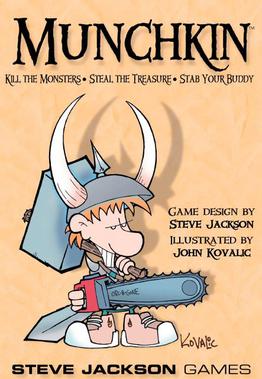
Munchkin Card Game

Rules may be inconsistent … so …

Any other disputes should be settled by loud arguments, with the owner of the game having the last word.

Munckin Rules (Jackson, 2001)

A Tautology

Self-governing systems cannot refer to external arbitration.

The No-Barber Principle

Russell’s Barber Paradox:

Barber shaves all who don’t shave themselves

Does the barber shave themselves?

Paradox: Definition includes itself in scope

No External Adjudicators

Forbidden:

External observer
Pre-specified outcome space/Hamiltonian
Privileged decomposition
External time parameter

No appeal to structure outside the game

That’s the sort of thing we want to forbid. And that’s what motivates the no-barber principle. The no-barber principle basically says we want to be in a situation where there are no external adjudicators. That means no external observer, no predefined outcome space, no external time parameter, and no privileged decomposition in the game. Nothing dictated from outside. And I’ll give you a very disconnected sense of how this manifests. Imagine if you had an external time parameter in the game, and as part of that game an entity’s time parameter was manipulated so it could move in time. A time travel paradox has the same impredicative circularity feel as Russell’s paradox — went back in time, met your mother, do you continue to exist? And that seems to come from someone outside the system playing with the time. If something emerged consistently inside the system, that shouldn’t be able to happen. So the idea is to create a game where you’re not appealing to any structure outside the game.

Baez-Fritz-Leinster Characterization of Information Loss

Baez et al. (2011):

Entropy from category theory
Three axioms uniquely determine information loss
No probability needed initially

The Three Axioms

\[F(f \circ g) = F(f) + F(g)\]

Information loss is additive
Compose processes → add losses

Convex Linearity

\[F(\lambda f \oplus (1-\lambda)g) = \lambda F(f) + (1-\lambda)F(g)\]

Probabilistic mixture of processes
Linear in probability weights

Continuity

Small change in process
Small change in information loss
\(F(f)\) continuous in \(f\)

The Main Result

Three axioms \(\Rightarrow\) unique form: \[F(f) = c(H(p) - H(q))\]

Information loss = scaled entropy difference
Shannon entropy emerges from axioms
No other measure satisfies all three

The Inaccessible Game Setup

Avoid external structure.
Represent information loss
Enforce information conservation

Information Isolation

Define information loss
Isolate game from observation/interaction
No external observer can extract or inject information

Marginal Entropy Conservation

\[ \sum_{i=1}^N h_i = C \]

Isolation: cf energy conservation — but for information

The Classical Observer

The Classical Observer - Correlated

The Classical Observer - Anti-correlated

Conceptually, imagine a classic physics setup where you can see inside a box: there are a number of particles moving around, sampled from random Gaussians. If you plot their velocities, they sit within a circle. In this case, the marginal \(h_i\) would be their velocity in each direction. The marginal distribution in each direction is Gaussian. Now, if the particles are correlated — everything tending to move in one diagonal direction — interestingly, the marginal entropies are the same. Although these are correlated, I’m not saying anything about the correlation when I conserve the marginal entropies, because if you look at the marginal distribution in each direction, it’s the same as in the uncorrelated case. And if they’re anti-correlated, it’s the same again. So I’m not making any statements about independence with this constraint.

The Classical Observer - Inaccessible

Joint Entropy

We don’t see see the outcome space
But we know it has a joint entropy

The \(I + H = C\) Structure

\[ \sum_{i=1}^N h_i = C \]

What does this conservation imply for dynamics?

Multi-Information: Measuring Correlation

\[ I = \sum_{i=1}^N h_i - H \]

‘Information Action’

\[ I + H = C \]

Conserved quantity splits into two parts

Analogy to classical mechanics

Energy: \(V + T = E\)
Information: \(I + H = C\)
System “rolls downhill” from correlation to disorder

Entropy Configuration Mapping

The Entropy Ladder

The Exponential Family

\[ p(\mathbf{ y}|\boldsymbol{ \theta}) = \exp\!\left(\boldsymbol{ \theta}^\top T(\mathbf{ y}) - \psi(\boldsymbol{ \theta})\right) \]

\(\boldsymbol{ \theta}\): natural parameters
\(\psi(\cdot)\): cumulant generating function
\(G(\boldsymbol{ \theta}) = \nabla^2\psi(\boldsymbol{ \theta})\): Fisher information

Axiomatically Distinguished

A choice is axiomatically distinguished if it is uniquely identifiable within the game’s axioms — without external structure such as Hamiltonians, clocks, or coordinates.

Maximum Entropy Production

Maximum entropy production: unique in Fisher metric
Constraint: marginal entropy conservation

Maximum Entropy Production

Maximise \[ \frac{\text{d}H}{\text{d}\tau} \] subject to \(\sum_i h_i = C\)

Constrained Entropy Ascent

Entropy via the Log-Partition Function

\[H(\boldsymbol{\theta}) = \psi(\boldsymbol{\theta}) - \boldsymbol{\theta}\cdot\nabla\psi(\boldsymbol{\theta})\]

\(\psi(\boldsymbol{\theta})\): log-partition function (CGF)
\(\boldsymbol{\eta} = \nabla\psi\): moment parameters \(\eta_k = \mathbb{E}[f_k]\)
\(G(\boldsymbol{\theta}) = \nabla^2\psi\): Fisher information matrix

Natural Gradient of Entropy

\[\nabla_{\!\boldsymbol{\theta}} H = -G(\boldsymbol{\theta})\boldsymbol{\theta}\]

Natural gradient: \[\nabla^{\mathrm{nat}} H = G^{-1}\nabla_{\!\boldsymbol{\theta}} H = -\boldsymbol{\theta}\]

Steepest entropy ascent \(\Rightarrow\) \(\dot{\boldsymbol{\theta}} \propto -\boldsymbol{\theta}\)
Descent in natural parameters — the symmetric part

Constrained Natural Gradient Dynamics

\[\dot{\boldsymbol{\theta}} = -\boldsymbol{\theta} + \nu(\tau)\,G^{-1}(\boldsymbol{\theta}) \mathbf{a}(\boldsymbol{\theta})\]

\(\mathbf{a}(\boldsymbol{\theta}) = \nabla_{\!\boldsymbol{\theta}}\!\sum_i h_i\) — constraint gradient.

\[\nu(\tau) = \frac{\mathbf{a}^\top\boldsymbol{\theta}}{\mathbf{a}^\top G^{-1}\mathbf{a}}\]

GENERIC-like Structure

Linearise around \(\boldsymbol{\theta}^*\)
\(\mathbf{q} = \boldsymbol{\theta} - \boldsymbol{\theta}^*\)

Linearised Flow

\[\dot{\mathbf{q}} = M\mathbf{q}\] where \(M = S + A\)

\(S\) is symmetric and irreversible (entropy production)
\(A\) is antisymmetric and reversible (entropy-conserving)

Information Relaxation Dynamics

Classical Obstruction at the Origin

Boundary Condition \[ I = C, \quad H = 0 \]
Conditional Shannon entropies always \(\geq 0\).
Prohibits \(H=0\) with positive marginals.

Von Neumann Entropy Resolution

Entanglement leads to negative conditional entropy.
Pure entangled state: \[ S(\rho_{AB}) = 0, \quad S(\rho_A) > 0, \quad S(\rho_B) > 0 \]

Information Loss Axioms

Provided by Parzygnat (2022) (quantum analogue of Baez et al. (2011))

The Matrix Exponential Family

\[ \rho(\boldsymbol{\theta}) = \exp\!\left(\sum_k \theta_k F_k - \psi(\boldsymbol{\theta})\,\mathbf{I}\right) \]

\(\boldsymbol{\theta}\): natural parameters
\(\psi(\boldsymbol{\theta}) = \log\,\mathrm{tr}\exp\!\left(\sum_k\theta_k F_k\right)\): cumulant generating function
\(G(\boldsymbol{\theta}) = \nabla^2\psi(\boldsymbol{\theta})\): BKM metric (quantum Fisher information)

Faithful States

Implies faithful states (full rank \(\rho\))
Pure states are on boundary of family
BKM Metric is divergent

The LME Origin

Globally pure state: \(S(\rho)=0\)
\(C = C_{\max} = \sum_i \log d_i\) (axiomatically distinguished)
Implies each marginal maximally mixed: \(s_i = \log d_i\)

Constraint Saturation and the Gibbs Lock

Marginal entropies linked: \(s_1 + s_2 = C\) (conserved sum)
Individual ceilings: \(s_i \leq \log d_i\)
Trade-off: as one marginal rises, the other must fall

Linked Marginal Entropies

Saturation and Second Order

At \(C=C_{\max}\): every \(s_i = \log d_i\) — each at its individual ceiling
Marginals locked: \(s_i(\tau) = \log d_i\) for all time

Saturation of Constraint

First-order condition vacuous
Admissible velocities: \(\dot{\boldsymbol{\theta}}\in \ker\nabla^2 \sum_i h_i\)

GENERIC Dynamics at the Origin

At the LME origin, constraint geometry produces a GENERIC decomposition (Lawrence, 2026):

Reversible (Lax): \(\dot{\rho} = -\mathrm{i}[K,\rho]\) — von Neumann equation emerges
Irreversible (SEA): steepest entropy ascent in marginal-preserving subspace

The Origin is Unreachable

\(\|\boldsymbol{\theta}\|\to\infty\) as \(\rho\to\rho_{\text{pure}}\)
Fisher (BKM) metric degenerates at boundary
Infinite Fisher distance — never literally reached
Trajectory distinguished by its asymptotic origin, not a literal start

Entropy Time

Need: an internal clock — external clocks forbidden by isolation
Game time \(\tau\): affine parameter, degenerates at origin

Entropy Time

\[\frac{\text{d}S}{\text{d}t} = c \quad \text{(constant entropy production)}\]

1 unit of \(t\) = \(c\) nats of entropy produced
No external clock, temperature, or Hamiltonian
Progress measured by entropy produced

From Information Geometry to Hamiltonian Mechanics

No imposed Hamiltonian
Can it be back-fitted from the game’s oscillating modes?
Saturation: all marginals pinned to maximally mixed states (Work in preparation)

Saturation and the Correlation Sector

Saturation pins every marginal: \(\rho_k = I/d_k\)
Correlation sector \(\mathcal{C} = \ker(\operatorname{tr}_{\neq k})\ \forall k\)
Reversible dynamics: compressed commutator \(L_\kappa\) on \(\mathcal{C}\)

The Ritz Criterion: Back-fitting a Hamiltonian

Ritz combination rule \(\omega_{ik} = \omega_{ij} + \omega_{jk}\)
- a flatness condition
Back-fitted Hamiltonian iff connection is exact (vertex potential exists)
This is the criterion, not an assumption

Conclusions

No barber principle
Information isolation
Axiomatic selection
Emergent effective rules

So to summarise: starting from a tautology — self-governing systems can’t appeal to external arbitration — and applying information theory, you get a surprisingly specific set of conclusions. The no-barber principle rules out external outcome spaces, clocks, Hamiltonians, and observers as primitives. Information isolation gives you a conservation law for marginal entropies. The requirement for a pure-state origin with positive marginals forces you into quantum probability — you can’t stay classical. The GENERIC structure and entropy time emerge from the dynamics. And the idea is that a Hamiltonian would have to emerge conditionally, in Gibbs-locked regions.

There are three papers now: the inaccessible game sets up the framework and derives the GENERIC structure. The origin paper derives the necessity of quantum probability. And the Hamiltonian paper derives the emergence of Hamiltonian dynamics from the Gibbs-locked region. Each paper has a “work in progress” quality — I’m not claiming these are complete. What I hope to have shown is that the tautology is not empty: it has mathematical teeth.

I was told I should finish with a question. Here’s mine: can we show that quantum mechanics — density matrices, von Neumann entropy, unitary evolution, Gibbs states — is, within the assumptions of the no-barber programme, the unique internally consistent language for a self-governing system that enforces information isolation? I don’t know the answer yet, but I think it’s the right question to be asking.

Thanks!

References

Baez, J.C., Fritz, T., Leinster, T., 2011. A characterization of entropy in terms of information loss. Entropy 13, 1945–1957. https://doi.org/10.3390/e13111945

Jackson, S., 2001. Munchkin. Steve Jackson Games.

Lawrence, N.D., 2026. The origin of the inaccessible game. https://doi.org/10.48550/arXiv.2601.12576

Parzygnat, A.J., 2022. A functorial characterization of von Neumann entropy. Cahiers de Topologie et Géométrie Différentielle Catégoriques 63, 89–128.