Reviewer Calibration for NIPS
There’s a Jupyter notebook implementing this approach available on github here or in Google Colab here.
One issue that can occur for a conference is differences in interpretation of the reviewing scale. For a number of years (dating back to at least NIPS 2002) mis-calibration between reviewers has been corrected for with a model. Area chairs see not just the actual scores of the paper, but also ‘corrected scores’. Both are used in the decision making process.
Reviewer calibration at NIPS dates back to a model first implemented in 2002 by John Platt when he was an area chair. It’s a regularized least squares model that Chris Burges and John wrote up in 2012. They’ve kindly made their write up available here.
Calibrated scores are used alongside original scores to help in judging the quality of papers.
We also knew that Zoubin and Max had modified the model last year, along with their program manager Hong Ge. However, before going through the previous work we first of all approached the question independently. However, the model we came up with turned out to be pretty much identical to that of Hong, Zoubin and Max, and the approach we are using to compute probability of accepts was also identical. The model is a probabilistic reinterpretation of the Platt and Burges model: one that treats the bias parameters and quality parameters as latent variables that are normally distributed. Marginalizing out the latent variables leads to an ANOVA style description of the data.
The Model
Our assumption is that the score from the $j$th reviewer for the $i$th paper is given by
\[y_{i,j} = f_i + b_j + \epsilon_{i, j}\]where $f_i$ is the objective quality of paper $i$ and $b_j$ is an offset associated with reviewer $j$. $\epsilon_{i,j}$ is a subjective quality estimate which reflects how a specific reviewer’s opinion differs from other reviewers (such differences in opinion may be due to differing expertise or perspective). The underlying ‘objective quality’ of the paper is assumed to be the same for all reviewers and the reviewer offset is assumed to be the same for all papers.
If we have $n$ papers and $m$ reviewers then this implies $n$ + $m$ + $nm$ values need to be estimated. Of course, in practice, the matrix is sparse, and we have no way of estimating the subjective quality for paper-reviewer pairs where no assignment was made. However, we can firstly assume that the subjective quality is drawn from a normal density with variance $\sigma^2$
\[\epsilon_{i, j} \sim N(0, \sigma^2 \mathbf{I})\]which reduces us to $n$ + $m$ + 1 parameters. The Platt-Burges model then estimated these parameters by regularized least squares. Instead, we follow Zoubin, Max and Hong’s approach of treating these values as latent variables. We assume that the objective quality, $f_i$, is also normally distributed with mean $\mu$ and variance $\alpha_f$,
\[f_i \sim N(\mu, \alpha_f)\]this now reduces us to $m$+3 parameters. However, we only have approximately $4m$ observations (4 papers per reviewer) so parameters may still not be that well determined (particularly for those reviewers that have only one review). We therefore also assume that the reviewer offset is a zero mean normally distributed latent variable,
\[b_j \sim N(0, \alpha_b),\]leaving us only four parameters: $\mu$, $\sigma^2$, $\alpha_f$ and $\alpha_b$. When we combine these assumptions together we see that our model assumes that any given review score is a combination of 3 normally distributed factors: the objective quality of the paper (variance $\alpha_f$), the subjective quality of the paper (variance $\sigma^2$) and the reviewer offset (variance $\alpha_b$). The a priori marginal variance of a reviewer-paper assignment’s score is the sum of these three components. Cross-correlations between reviewer-paper assignments occur if either the reviewer is the same (when the cross covariance is given by $\alpha_b$) or the paper is the same (when the cross covariance is given by $\alpha_f$). With a constant mean coming from the mean of the ‘subjective quality’, this gives us a joint model for reviewer scores as follows:
\[\mathbf{y} \sim N(\mu \mathbf{1}, \mathbf{K})\]where $\mathbf{y}$ is a vector of stacked scores $\mathbf{1}$ is the vector of ones and the elements of the covariance function are given by
\[k(i,j; k,l) = \delta_{i,k} \alpha_f + \delta_{j,l} \alpha_b + \delta_{i, k}\delta_{j,l} \sigma^2\]where $i$ and $j$ are the index of the paper and reviewer in the rows of $\mathbf{K}$ and $k$ and $l$ are the index of the paper and reviewer in the columns of $\mathbf{K}$.
It can be convenient to reparameterize slightly into an overall scale $\alpha_f$, and normalized variance parameters,
\[k(i,j; k,l) = \alpha_f(\delta_{i,k} + \delta_{j,l} \frac{\alpha_b}{\alpha_f} + \delta_{i, k}\delta_{j,l} \frac{\sigma^2}{\alpha_f})\]which we rewrite to give two ratios: offset/objective quality ratio, $\hat{\alpha}_b$ and subjective/objective ratio $\hat{\sigma}^2$ ratio.
\[k(i,j; k,l) = \alpha_f(\delta_{i,k} + \delta_{j,l} \hat{\alpha}_b + \delta_{i, k}\delta_{j,l} \hat{\sigma}^2)\]The advantage of this parameterization is it allows us to optimize $\alpha_f$ directly through maximum likelihood (with a fixed point equation). This leaves us with two free parameters, that we might explore on a grid.
We expect both $\mu$ and $\alpha_f$ to be very well determined due to the number of observations in the data. The negative log likelihood is
\[\frac{\|\mathbf{y}\|}{2}\log2\pi\alpha_f + \frac{1}{2}\log \left|\hat{\mathbf{K}}\right| + \frac{1}{2\alpha_f}\mathbf{y}^\top \hat{\mathbf{K}}^{-1} \mathbf{y}\]where $|\mathbf{y}|$ is the length of $\mathbf{y}$ (i.e. the number of reviews) and $\hat{\mathbf{K}}=\alpha_f^{-1}\mathbf{K}$ is the scale normalised covariance. This negative log likelihood is easily minimized to recover
\[\alpha_f = \frac{1}{\|\mathbf{y}\|} \mathbf{y}^\top \hat{\mathbf{K}}^{-1} \mathbf{y}\]A Bayesian analysis of $\alpha_f$ parameter is possible with gamma priors, but it would merely shows that this parameter is extremely well determined (the degrees of freedom parameter of the associated Student-$t$ marginal likelihood scales will the number of reviews, which will be around $|\mathbf{y}| \approx 6,000$ in our case.
We can set these parameters by maximum likelihood and then we can remove the offset from the model by computing the conditional distribution over the paper scores with the bias removed, $s_{i,j} = f_i + \epsilon_{i,j}$. This conditional distribution is found as
\[\mathbf{s}\|\mathbf{y}, \alpha_f,\alpha_b, \sigma^2 \sim N(\boldsymbol{\mu}_s, \boldsymbol{\Sigma}_s)\]where
\[\boldsymbol{\mu}_s = \mathbf{K}_s\mathbf{K}^{-1}\mathbf{y}\]and
\[\boldsymbol{\Sigma}_s = \mathbf{K}_s - \mathbf{K}_s\mathbf{K}^{-1}\mathbf{K}_s\]and $\mathbf{K}_s$ is the covariance associated with the quality terms only with elements given by,
\[k_s(i,j;k,l) = \delta_{i,k}(\alpha_f + \delta_{j,l}\sigma^2).\]We now use $\boldsymbol{\mu}_s$ (which is both the mode and the mean of the posterior over $\mathbf{s}$) as the calibrated quality score.
Analysis of Variance
The model above is a type of Gaussian process model with a specific covariance function (or kernel). The variances are highly interpretable though, because the covariance function is made up of a sum of effects. Studying these variances is known as analysis of variance in statistics, and is commonly used for batch effects. It is known as an ANOVA model. It is easy to extend this model to include batch effects such as whether or not the reviewer is a student or whether or not the reviewer has published at NIPS before. We will conduct these analyses in due course. Last year, Zoubin, Max and Hong explored whether the reviewer confidence could be included in the model, but they found it did not help with performance on hold out data.
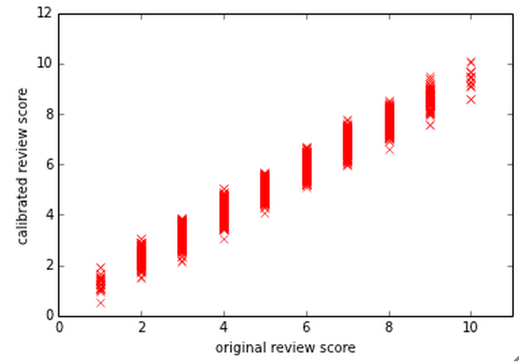
Scatter plot of Quality Score vs Calibrated Quality Score
Probability of Acceptance
To predict the probability of acceptance of any given paper, we sample from the multivariate normal that gives the posterior over $\mathbf{s}$. These samples are sorted according to the values of $\mathbf{s}$, and the top scoring papers are considered to be accepts. These samples are taken 1000 times and the probability of acceptance is computed for each paper by seeing how many times the paper received a positive outcome from the thousand samples.