Inducing Variable Demo

×

[jupyter][google colab]

Setup

pods

[edit]

In Sheffield we created a suite of software tools for ‘Open Data Science.’ Open data science is an approach to sharing code, models and data that should make it easier for companies, health professionals and scientists to gain access to data science techniques.

You can also check this blog post on Open Data Science.

The software can be installed using

%pip install --upgrade git+https://github.com/lawrennd/ods

from the command prompt where you can access your python installation.

The code is also available on github: https://github.com/lawrennd/ods

Once pods is installed, it can be imported in the usual manner.

import pods

mlai

[edit]

The mlai software is a suite of helper functions for teaching and demonstrating machine learning algorithms. It was first used in the Machine Learning and Adaptive Intelligence course in Sheffield in 2013.

The software can be installed using

%pip install --upgrade git+https://github.com/lawrennd/mlai.git

from the command prompt where you can access your python installation.

The code is also available on github: https://github.com/lawrennd/mlai

Once mlai is installed, it can be imported in the usual manner.

import mlai

%pip install gpy

GPy: A Gaussian Process Framework in Python

[edit]

Gaussian processes are a flexible tool for non-parametric analysis with uncertainty. The GPy software was started in Sheffield to provide a easy to use interface to GPs. One which allowed the user to focus on the modelling rather than the mathematics.

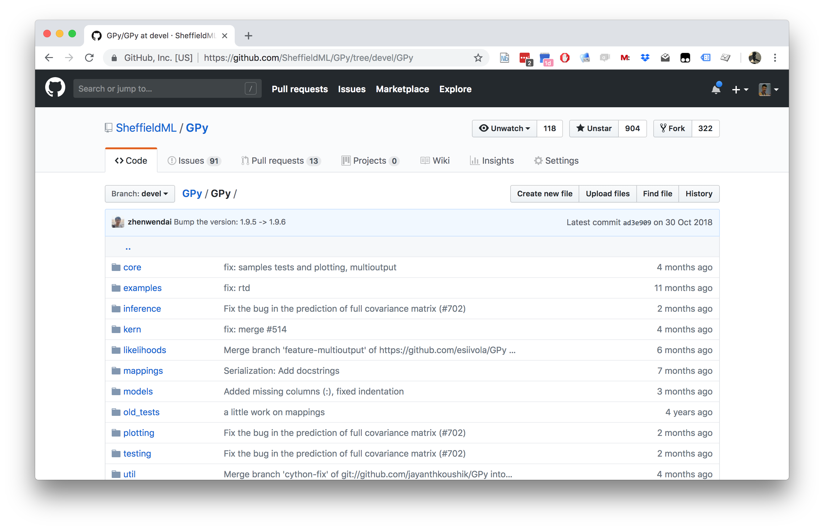
Figure: GPy is a BSD licensed software code base for implementing Gaussian process models in Python. It is designed for teaching and modelling. We welcome contributions which can be made through the Github repository https://github.com/SheffieldML/GPy

GPy is a BSD licensed software code base for implementing Gaussian process models in python. This allows GPs to be combined with a wide variety of software libraries.

The software itself is available on GitHub and the team welcomes contributions.

The aim for GPy is to be a probabilistic-style programming language, i.e. you specify the model rather than the algorithm. As well as a large range of covariance functions the software allows for non-Gaussian likelihoods, multivariate outputs, dimensionality reduction and approximations for larger data sets.

The documentation for GPy can be found here.

A Simple Regression Problem

[edit]

Here we set up a simple one dimensional regression problem. The input locations, \(\mathbf{X}\), are in two separate clusters. The response variable, \(\mathbf{ y}\), is sampled from a Gaussian process with an exponentiated quadratic covariance.

import numpy as np
import GPy

np.random.seed(101)

N = 50
noise_var = 0.01
X = np.zeros((50, 1))
X[:25, :] = np.linspace(0,3,25)[:,None] # First cluster of inputs/covariates
X[25:, :] = np.linspace(7,10,25)[:,None] # Second cluster of inputs/covariates

# Sample response variables from a Gaussian process with exponentiated quadratic covariance.
k = GPy.kern.RBF(1)
y = np.random.multivariate_normal(np.zeros(N),k.K(X)+np.eye(N)*np.sqrt(noise_var)).reshape(-1,1)

First we perform a full Gaussian process regression on the data. We create a GP model, m_full, and fit it to the data, plotting the resulting fit.

m_full = GPy.models.GPRegression(X,y)
_ = m_full.optimize(messages=True) # Optimize parameters of covariance function

Figure: Full Gaussian process fitted to the data set.

Now we set up the inducing variables, \(\mathbf{u}\). Each inducing variable has its own associated input index, \(\mathbf{Z}\), which lives in the same space as \(\mathbf{X}\). Here we are using the true covariance function parameters to generate the fit.

kern = GPy.kern.RBF(1)
Z = np.hstack(
        (np.linspace(2.5,4.,3),
        np.linspace(7,8.5,3)))[:,None]
m = GPy.models.SparseGPRegression(X,y,kernel=kern,Z=Z)
m.noise_var = noise_var
m.inducing_inputs.constrain_fixed()
display(m)

Figure: Sparse Gaussian process fitted with six inducing variables, no optimization of parameters or inducing variables.

_ = m.optimize(messages=True)
display(m)

Figure: Gaussian process fitted with inducing variables fixed and parameters optimized

m.randomize()
m.inducing_inputs.unconstrain()
_ = m.optimize(messages=True)

Figure: Gaussian process fitted with location of inducing variables and parameters both optimized

Now we will vary the number of inducing points used to form the approximation.

m.num_inducing=8
m.randomize()
M = 8
m.set_Z(np.random.rand(M,1)*12)

_ = m.optimize(messages=True)

Figure: Comparison of the full Gaussian process fit with a sparse Gaussian process using eight inducing varibles. Both inducing variables and parameters are optimized.

And we can compare the probability of the result to the full model.

print(m.log_likelihood(), m_full.log_likelihood())

References