$$\newcommand{\tk}[1]{}
\newcommand{\Amatrix}{\mathbf{A}}
\newcommand{\KL}[2]{\text{KL}\left( #1\,\|\,#2 \right)}
\newcommand{\Kaast}{\kernelMatrix_{\mathbf{ \ast}\mathbf{ \ast}}}
\newcommand{\Kastu}{\kernelMatrix_{\mathbf{ \ast} \inducingVector}}
\newcommand{\Kff}{\kernelMatrix_{\mappingFunctionVector \mappingFunctionVector}}
\newcommand{\Kfu}{\kernelMatrix_{\mappingFunctionVector \inducingVector}}
\newcommand{\Kuast}{\kernelMatrix_{\inducingVector \bf\ast}}
\newcommand{\Kuf}{\kernelMatrix_{\inducingVector \mappingFunctionVector}}
\newcommand{\Kuu}{\kernelMatrix_{\inducingVector \inducingVector}}
\newcommand{\Kuui}{\Kuu^{-1}}
\newcommand{\Qaast}{\mathbf{Q}_{\bf \ast \ast}}
\newcommand{\Qastf}{\mathbf{Q}_{\ast \mappingFunction}}
\newcommand{\Qfast}{\mathbf{Q}_{\mappingFunctionVector \bf \ast}}
\newcommand{\Qff}{\mathbf{Q}_{\mappingFunctionVector \mappingFunctionVector}}
\newcommand{\aMatrix}{\mathbf{A}}
\newcommand{\aScalar}{a}
\newcommand{\aVector}{\mathbf{a}}
\newcommand{\acceleration}{a}
\newcommand{\bMatrix}{\mathbf{B}}
\newcommand{\bScalar}{b}
\newcommand{\bVector}{\mathbf{b}}
\newcommand{\basisFunc}{\phi}
\newcommand{\basisFuncVector}{\boldsymbol{ \basisFunc}}
\newcommand{\basisFunction}{\phi}
\newcommand{\basisLocation}{\mu}
\newcommand{\basisMatrix}{\boldsymbol{ \Phi}}
\newcommand{\basisScalar}{\basisFunction}
\newcommand{\basisVector}{\boldsymbol{ \basisFunction}}
\newcommand{\activationFunction}{\phi}
\newcommand{\activationMatrix}{\boldsymbol{ \Phi}}
\newcommand{\activationScalar}{\basisFunction}
\newcommand{\activationVector}{\boldsymbol{ \basisFunction}}
\newcommand{\bigO}{\mathcal{O}}
\newcommand{\binomProb}{\pi}
\newcommand{\cMatrix}{\mathbf{C}}
\newcommand{\cbasisMatrix}{\hat{\boldsymbol{ \Phi}}}
\newcommand{\cdataMatrix}{\hat{\dataMatrix}}
\newcommand{\cdataScalar}{\hat{\dataScalar}}
\newcommand{\cdataVector}{\hat{\dataVector}}
\newcommand{\centeredKernelMatrix}{\mathbf{ \MakeUppercase{\centeredKernelScalar}}}
\newcommand{\centeredKernelScalar}{b}
\newcommand{\centeredKernelVector}{\centeredKernelScalar}
\newcommand{\centeringMatrix}{\mathbf{H}}
\newcommand{\chiSquaredDist}[2]{\chi_{#1}^{2}\left(#2\right)}
\newcommand{\chiSquaredSamp}[1]{\chi_{#1}^{2}}
\newcommand{\conditionalCovariance}{\boldsymbol{ \Sigma}}
\newcommand{\coregionalizationMatrix}{\mathbf{B}}
\newcommand{\coregionalizationScalar}{b}
\newcommand{\coregionalizationVector}{\mathbf{ \coregionalizationScalar}}
\newcommand{\covDist}[2]{\text{cov}_{#2}\left(#1\right)}
\newcommand{\covSamp}[1]{\text{cov}\left(#1\right)}
\newcommand{\covarianceScalar}{c}
\newcommand{\covarianceVector}{\mathbf{ \covarianceScalar}}
\newcommand{\covarianceMatrix}{\mathbf{C}}
\newcommand{\covarianceMatrixTwo}{\boldsymbol{ \Sigma}}
\newcommand{\croupierScalar}{s}
\newcommand{\croupierVector}{\mathbf{ \croupierScalar}}
\newcommand{\croupierMatrix}{\mathbf{ \MakeUppercase{\croupierScalar}}}
\newcommand{\dataDim}{p}
\newcommand{\dataIndex}{i}
\newcommand{\dataIndexTwo}{j}
\newcommand{\dataMatrix}{\mathbf{Y}}
\newcommand{\dataScalar}{y}
\newcommand{\dataSet}{\mathcal{D}}
\newcommand{\dataStd}{\sigma}
\newcommand{\dataVector}{\mathbf{ \dataScalar}}
\newcommand{\decayRate}{d}
\newcommand{\degreeMatrix}{\mathbf{ \MakeUppercase{\degreeScalar}}}
\newcommand{\degreeScalar}{d}
\newcommand{\degreeVector}{\mathbf{ \degreeScalar}}
\newcommand{\diag}[1]{\text{diag}\left(#1\right)}
\newcommand{\diagonalMatrix}{\mathbf{D}}
\newcommand{\diff}[2]{\frac{\text{d}#1}{\text{d}#2}}
\newcommand{\diffTwo}[2]{\frac{\text{d}^2#1}{\text{d}#2^2}}
\newcommand{\displacement}{x}
\newcommand{\displacementVector}{\textbf{\displacement}}
\newcommand{\distanceMatrix}{\mathbf{ \MakeUppercase{\distanceScalar}}}
\newcommand{\distanceScalar}{d}
\newcommand{\distanceVector}{\mathbf{ \distanceScalar}}
\newcommand{\eigenvaltwo}{\ell}
\newcommand{\eigenvaltwoMatrix}{\mathbf{L}}
\newcommand{\eigenvaltwoVector}{\mathbf{l}}
\newcommand{\eigenvalue}{\lambda}
\newcommand{\eigenvalueMatrix}{\boldsymbol{ \Lambda}}
\newcommand{\eigenvalueVector}{\boldsymbol{ \lambda}}
\newcommand{\eigenvector}{\mathbf{ \eigenvectorScalar}}
\newcommand{\eigenvectorMatrix}{\mathbf{U}}
\newcommand{\eigenvectorScalar}{u}
\newcommand{\eigenvectwo}{\mathbf{v}}
\newcommand{\eigenvectwoMatrix}{\mathbf{V}}
\newcommand{\eigenvectwoScalar}{v}
\newcommand{\entropy}[1]{\mathcal{H}\left(#1\right)}
\newcommand{\errorFunction}{E}
\newcommand{\expDist}[2]{\left\langle#1\right\rangle_{#2}}
\newcommand{\expSamp}[1]{\left\langle#1\right\rangle}
\newcommand{\expectation}[1]{\left\langle #1 \right\rangle }
\newcommand{\expectationDist}[2]{\left\langle #1 \right\rangle _{#2}}
\newcommand{\expectedDistanceMatrix}{\mathcal{D}}
\newcommand{\eye}{\mathbf{I}}
\newcommand{\fantasyDim}{r}
\newcommand{\fantasyMatrix}{\mathbf{ \MakeUppercase{\fantasyScalar}}}
\newcommand{\fantasyScalar}{z}
\newcommand{\fantasyVector}{\mathbf{ \fantasyScalar}}
\newcommand{\featureStd}{\varsigma}
\newcommand{\gammaCdf}[3]{\mathcal{GAMMA CDF}\left(#1|#2,#3\right)}
\newcommand{\gammaDist}[3]{\mathcal{G}\left(#1|#2,#3\right)}
\newcommand{\gammaSamp}[2]{\mathcal{G}\left(#1,#2\right)}
\newcommand{\gaussianDist}[3]{\mathcal{N}\left(#1|#2,#3\right)}
\newcommand{\gaussianSamp}[2]{\mathcal{N}\left(#1,#2\right)}
\newcommand{\uniformDist}[3]{\mathcal{U}\left(#1|#2,#3\right)}
\newcommand{\uniformSamp}[2]{\mathcal{U}\left(#1,#2\right)}
\newcommand{\given}{|}
\newcommand{\half}{\frac{1}{2}}
\newcommand{\heaviside}{H}
\newcommand{\hiddenMatrix}{\mathbf{ \MakeUppercase{\hiddenScalar}}}
\newcommand{\hiddenScalar}{h}
\newcommand{\hiddenVector}{\mathbf{ \hiddenScalar}}
\newcommand{\identityMatrix}{\eye}
\newcommand{\inducingInputScalar}{z}
\newcommand{\inducingInputVector}{\mathbf{ \inducingInputScalar}}
\newcommand{\inducingInputMatrix}{\mathbf{Z}}
\newcommand{\inducingScalar}{u}
\newcommand{\inducingVector}{\mathbf{ \inducingScalar}}
\newcommand{\inducingMatrix}{\mathbf{U}}
\newcommand{\inlineDiff}[2]{\text{d}#1/\text{d}#2}
\newcommand{\inputDim}{q}
\newcommand{\inputMatrix}{\mathbf{X}}
\newcommand{\inputScalar}{x}
\newcommand{\inputSpace}{\mathcal{X}}
\newcommand{\inputVals}{\inputVector}
\newcommand{\inputVector}{\mathbf{ \inputScalar}}
\newcommand{\iterNum}{k}
\newcommand{\kernel}{\kernelScalar}
\newcommand{\kernelMatrix}{\mathbf{K}}
\newcommand{\kernelScalar}{k}
\newcommand{\kernelVector}{\mathbf{ \kernelScalar}}
\newcommand{\kff}{\kernelScalar_{\mappingFunction \mappingFunction}}
\newcommand{\kfu}{\kernelVector_{\mappingFunction \inducingScalar}}
\newcommand{\kuf}{\kernelVector_{\inducingScalar \mappingFunction}}
\newcommand{\kuu}{\kernelVector_{\inducingScalar \inducingScalar}}
\newcommand{\lagrangeMultiplier}{\lambda}
\newcommand{\lagrangeMultiplierMatrix}{\boldsymbol{ \Lambda}}
\newcommand{\lagrangian}{L}
\newcommand{\laplacianFactor}{\mathbf{ \MakeUppercase{\laplacianFactorScalar}}}
\newcommand{\laplacianFactorScalar}{m}
\newcommand{\laplacianFactorVector}{\mathbf{ \laplacianFactorScalar}}
\newcommand{\laplacianMatrix}{\mathbf{L}}
\newcommand{\laplacianScalar}{\ell}
\newcommand{\laplacianVector}{\mathbf{ \ell}}
\newcommand{\latentDim}{q}
\newcommand{\latentDistanceMatrix}{\boldsymbol{ \Delta}}
\newcommand{\latentDistanceScalar}{\delta}
\newcommand{\latentDistanceVector}{\boldsymbol{ \delta}}
\newcommand{\latentForce}{f}
\newcommand{\latentFunction}{u}
\newcommand{\latentFunctionVector}{\mathbf{ \latentFunction}}
\newcommand{\latentFunctionMatrix}{\mathbf{ \MakeUppercase{\latentFunction}}}
\newcommand{\latentIndex}{j}
\newcommand{\latentScalar}{z}
\newcommand{\latentVector}{\mathbf{ \latentScalar}}
\newcommand{\latentMatrix}{\mathbf{Z}}
\newcommand{\learnRate}{\eta}
\newcommand{\lengthScale}{\ell}
\newcommand{\rbfWidth}{\ell}
\newcommand{\likelihoodBound}{\mathcal{L}}
\newcommand{\likelihoodFunction}{L}
\newcommand{\locationScalar}{\mu}
\newcommand{\locationVector}{\boldsymbol{ \locationScalar}}
\newcommand{\locationMatrix}{\mathbf{M}}
\newcommand{\variance}[1]{\text{var}\left( #1 \right)}
\newcommand{\mappingFunction}{f}
\newcommand{\mappingFunctionMatrix}{\mathbf{F}}
\newcommand{\mappingFunctionTwo}{g}
\newcommand{\mappingFunctionTwoMatrix}{\mathbf{G}}
\newcommand{\mappingFunctionTwoVector}{\mathbf{ \mappingFunctionTwo}}
\newcommand{\mappingFunctionVector}{\mathbf{ \mappingFunction}}
\newcommand{\scaleScalar}{s}
\newcommand{\mappingScalar}{w}
\newcommand{\mappingVector}{\mathbf{ \mappingScalar}}
\newcommand{\mappingMatrix}{\mathbf{W}}
\newcommand{\mappingScalarTwo}{v}
\newcommand{\mappingVectorTwo}{\mathbf{ \mappingScalarTwo}}
\newcommand{\mappingMatrixTwo}{\mathbf{V}}
\newcommand{\maxIters}{K}
\newcommand{\meanMatrix}{\mathbf{M}}
\newcommand{\meanScalar}{\mu}
\newcommand{\meanTwoMatrix}{\mathbf{M}}
\newcommand{\meanTwoScalar}{m}
\newcommand{\meanTwoVector}{\mathbf{ \meanTwoScalar}}
\newcommand{\meanVector}{\boldsymbol{ \meanScalar}}
\newcommand{\mrnaConcentration}{m}
\newcommand{\naturalFrequency}{\omega}
\newcommand{\neighborhood}[1]{\mathcal{N}\left( #1 \right)}
\newcommand{\neilurl}{http://inverseprobability.com/}
\newcommand{\noiseMatrix}{\boldsymbol{ E}}
\newcommand{\noiseScalar}{\epsilon}
\newcommand{\noiseVector}{\boldsymbol{ \epsilon}}
\newcommand{\noiseStd}{\sigma}
\newcommand{\norm}[1]{\left\Vert #1 \right\Vert}
\newcommand{\normalizedLaplacianMatrix}{\hat{\mathbf{L}}}
\newcommand{\normalizedLaplacianScalar}{\hat{\ell}}
\newcommand{\normalizedLaplacianVector}{\hat{\mathbf{ \ell}}}
\newcommand{\numActive}{m}
\newcommand{\numBasisFunc}{m}
\newcommand{\numComponents}{m}
\newcommand{\numComps}{K}
\newcommand{\numData}{n}
\newcommand{\numFeatures}{K}
\newcommand{\numHidden}{h}
\newcommand{\numInducing}{m}
\newcommand{\numLayers}{\ell}
\newcommand{\numNeighbors}{K}
\newcommand{\numSequences}{s}
\newcommand{\numSuccess}{s}
\newcommand{\numTasks}{m}
\newcommand{\numTime}{T}
\newcommand{\numTrials}{S}
\newcommand{\outputIndex}{j}
\newcommand{\paramVector}{\boldsymbol{ \theta}}
\newcommand{\parameterMatrix}{\boldsymbol{ \Theta}}
\newcommand{\parameterScalar}{\theta}
\newcommand{\parameterVector}{\boldsymbol{ \parameterScalar}}
\newcommand{\partDiff}[2]{\frac{\partial#1}{\partial#2}}
\newcommand{\precisionScalar}{j}
\newcommand{\precisionVector}{\mathbf{ \precisionScalar}}
\newcommand{\precisionMatrix}{\mathbf{J}}
\newcommand{\pseudotargetScalar}{\widetilde{y}}
\newcommand{\pseudotargetVector}{\mathbf{ \pseudotargetScalar}}
\newcommand{\pseudotargetMatrix}{\mathbf{ \widetilde{Y}}}
\newcommand{\rank}[1]{\text{rank}\left(#1\right)}
\newcommand{\rayleighDist}[2]{\mathcal{R}\left(#1|#2\right)}
\newcommand{\rayleighSamp}[1]{\mathcal{R}\left(#1\right)}
\newcommand{\responsibility}{r}
\newcommand{\rotationScalar}{r}
\newcommand{\rotationVector}{\mathbf{ \rotationScalar}}
\newcommand{\rotationMatrix}{\mathbf{R}}
\newcommand{\sampleCovScalar}{s}
\newcommand{\sampleCovVector}{\mathbf{ \sampleCovScalar}}
\newcommand{\sampleCovMatrix}{\mathbf{s}}
\newcommand{\scalarProduct}[2]{\left\langle{#1},{#2}\right\rangle}
\newcommand{\sign}[1]{\text{sign}\left(#1\right)}
\newcommand{\sigmoid}[1]{\sigma\left(#1\right)}
\newcommand{\singularvalue}{\ell}
\newcommand{\singularvalueMatrix}{\mathbf{L}}
\newcommand{\singularvalueVector}{\mathbf{l}}
\newcommand{\sorth}{\mathbf{u}}
\newcommand{\spar}{\lambda}
\newcommand{\trace}[1]{\text{tr}\left(#1\right)}
\newcommand{\BasalRate}{B}
\newcommand{\DampingCoefficient}{C}
\newcommand{\DecayRate}{D}
\newcommand{\Displacement}{X}
\newcommand{\LatentForce}{F}
\newcommand{\Mass}{M}
\newcommand{\Sensitivity}{S}
\newcommand{\basalRate}{b}
\newcommand{\dampingCoefficient}{c}
\newcommand{\mass}{m}
\newcommand{\sensitivity}{s}
\newcommand{\springScalar}{\kappa}
\newcommand{\springVector}{\boldsymbol{ \kappa}}
\newcommand{\springMatrix}{\boldsymbol{ \mathcal{K}}}
\newcommand{\tfConcentration}{p}
\newcommand{\tfDecayRate}{\delta}
\newcommand{\tfMrnaConcentration}{f}
\newcommand{\tfVector}{\mathbf{ \tfConcentration}}
\newcommand{\velocity}{v}
\newcommand{\sufficientStatsScalar}{g}
\newcommand{\sufficientStatsVector}{\mathbf{ \sufficientStatsScalar}}
\newcommand{\sufficientStatsMatrix}{\mathbf{G}}
\newcommand{\switchScalar}{s}
\newcommand{\switchVector}{\mathbf{ \switchScalar}}
\newcommand{\switchMatrix}{\mathbf{S}}
\newcommand{\tr}[1]{\text{tr}\left(#1\right)}
\newcommand{\loneNorm}[1]{\left\Vert #1 \right\Vert_1}
\newcommand{\ltwoNorm}[1]{\left\Vert #1 \right\Vert_2}
\newcommand{\onenorm}[1]{\left\vert#1\right\vert_1}
\newcommand{\twonorm}[1]{\left\Vert #1 \right\Vert}
\newcommand{\vScalar}{v}
\newcommand{\vVector}{\mathbf{v}}
\newcommand{\vMatrix}{\mathbf{V}}
\newcommand{\varianceDist}[2]{\text{var}_{#2}\left( #1 \right)}
\newcommand{\vecb}[1]{\left(#1\right):}
\newcommand{\weightScalar}{w}
\newcommand{\weightVector}{\mathbf{ \weightScalar}}
\newcommand{\weightMatrix}{\mathbf{W}}
\newcommand{\weightedAdjacencyMatrix}{\mathbf{A}}
\newcommand{\weightedAdjacencyScalar}{a}
\newcommand{\weightedAdjacencyVector}{\mathbf{ \weightedAdjacencyScalar}}
\newcommand{\onesVector}{\mathbf{1}}
\newcommand{\zerosVector}{\mathbf{0}}
$$
at NIPS Workshop on Statistical Methods for Understanding Neural Systems on Dec 11, 2015
[reveal]
Abstract
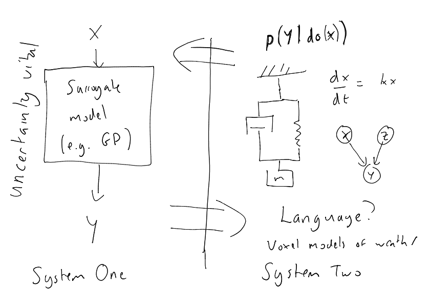
In this talk we will discuss how our current set of modelling solutions relates to dual process models from psychology. By analogising with layered models of networks we first address the danger of focussing purely on mechanism (or biological plausibility) when discussion modelling in the brain. We term this idea the mechanistic fallacy. In an attempt to operate at a higher level of abstraction, we then take a conceptual approach and attempt to map the broader domain of mechanistic and phenomological models to dual process ideas from psychology. It seems that System 1 is closer to phenomological and System 2 is closer to mechanistic ideas. We will draw connections to surrogate modelling (also known as emmulation) and speculate that one role of System 2 may be to provide additional simulation data for System 1.
Summary of the workshop can be found here: https://memming.wordpress.com/2015/12/15/nips-2015-workshops/
blog post on System
Zero.
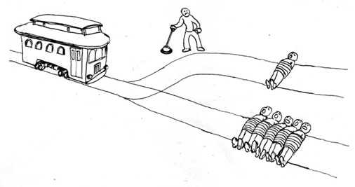
The Trolley Problem
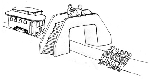
The Push and the Trolley
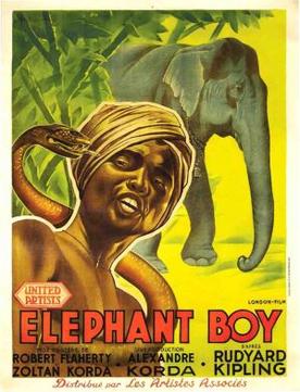
The Elephant and its Rider
The Righteous Mind
The Chimp Paradox
blog post on Artificial
Stupidity.
Thanks!
For more information on these subjects and more you might want to
check the following resources.
References