Machine Learning and the Physical World

Neil D. Lawrence

$$\newcommand{\tk}[1]{} \newcommand{\Amatrix}{\mathbf{A}} \newcommand{\KL}[2]{\text{KL}\left( #1\,\|\,#2 \right)} \newcommand{\Kaast}{\kernelMatrix_{\mathbf{ \ast}\mathbf{ \ast}}} \newcommand{\Kastu}{\kernelMatrix_{\mathbf{ \ast} \inducingVector}} \newcommand{\Kff}{\kernelMatrix_{\mappingFunctionVector \mappingFunctionVector}} \newcommand{\Kfu}{\kernelMatrix_{\mappingFunctionVector \inducingVector}} \newcommand{\Kuast}{\kernelMatrix_{\inducingVector \bf\ast}} \newcommand{\Kuf}{\kernelMatrix_{\inducingVector \mappingFunctionVector}} \newcommand{\Kuu}{\kernelMatrix_{\inducingVector \inducingVector}} \newcommand{\Kuui}{\Kuu^{-1}} \newcommand{\Qaast}{\mathbf{Q}_{\bf \ast \ast}} \newcommand{\Qastf}{\mathbf{Q}_{\ast \mappingFunction}} \newcommand{\Qfast}{\mathbf{Q}_{\mappingFunctionVector \bf \ast}} \newcommand{\Qff}{\mathbf{Q}_{\mappingFunctionVector \mappingFunctionVector}} \newcommand{\aMatrix}{\mathbf{A}} \newcommand{\aScalar}{a} \newcommand{\aVector}{\mathbf{a}} \newcommand{\acceleration}{a} \newcommand{\bMatrix}{\mathbf{B}} \newcommand{\bScalar}{b} \newcommand{\bVector}{\mathbf{b}} \newcommand{\basisFunc}{\phi} \newcommand{\basisFuncVector}{\boldsymbol{ \basisFunc}} \newcommand{\basisFunction}{\phi} \newcommand{\basisLocation}{\mu} \newcommand{\basisMatrix}{\boldsymbol{ \Phi}} \newcommand{\basisScalar}{\basisFunction} \newcommand{\basisVector}{\boldsymbol{ \basisFunction}} \newcommand{\activationFunction}{\phi} \newcommand{\activationMatrix}{\boldsymbol{ \Phi}} \newcommand{\activationScalar}{\basisFunction} \newcommand{\activationVector}{\boldsymbol{ \basisFunction}} \newcommand{\bigO}{\mathcal{O}} \newcommand{\binomProb}{\pi} \newcommand{\cMatrix}{\mathbf{C}} \newcommand{\cbasisMatrix}{\hat{\boldsymbol{ \Phi}}} \newcommand{\cdataMatrix}{\hat{\dataMatrix}} \newcommand{\cdataScalar}{\hat{\dataScalar}} \newcommand{\cdataVector}{\hat{\dataVector}} \newcommand{\centeredKernelMatrix}{\mathbf{ \MakeUppercase{\centeredKernelScalar}}} \newcommand{\centeredKernelScalar}{b} \newcommand{\centeredKernelVector}{\centeredKernelScalar} \newcommand{\centeringMatrix}{\mathbf{H}} \newcommand{\chiSquaredDist}[2]{\chi_{#1}^{2}\left(#2\right)} \newcommand{\chiSquaredSamp}[1]{\chi_{#1}^{2}} \newcommand{\conditionalCovariance}{\boldsymbol{ \Sigma}} \newcommand{\coregionalizationMatrix}{\mathbf{B}} \newcommand{\coregionalizationScalar}{b} \newcommand{\coregionalizationVector}{\mathbf{ \coregionalizationScalar}} \newcommand{\covDist}[2]{\text{cov}_{#2}\left(#1\right)} \newcommand{\covSamp}[1]{\text{cov}\left(#1\right)} \newcommand{\covarianceScalar}{c} \newcommand{\covarianceVector}{\mathbf{ \covarianceScalar}} \newcommand{\covarianceMatrix}{\mathbf{C}} \newcommand{\covarianceMatrixTwo}{\boldsymbol{ \Sigma}} \newcommand{\croupierScalar}{s} \newcommand{\croupierVector}{\mathbf{ \croupierScalar}} \newcommand{\croupierMatrix}{\mathbf{ \MakeUppercase{\croupierScalar}}} \newcommand{\dataDim}{p} \newcommand{\dataIndex}{i} \newcommand{\dataIndexTwo}{j} \newcommand{\dataMatrix}{\mathbf{Y}} \newcommand{\dataScalar}{y} \newcommand{\dataSet}{\mathcal{D}} \newcommand{\dataStd}{\sigma} \newcommand{\dataVector}{\mathbf{ \dataScalar}} \newcommand{\decayRate}{d} \newcommand{\degreeMatrix}{\mathbf{ \MakeUppercase{\degreeScalar}}} \newcommand{\degreeScalar}{d} \newcommand{\degreeVector}{\mathbf{ \degreeScalar}} \newcommand{\diag}[1]{\text{diag}\left(#1\right)} \newcommand{\diagonalMatrix}{\mathbf{D}} \newcommand{\diff}[2]{\frac{\text{d}#1}{\text{d}#2}} \newcommand{\diffTwo}[2]{\frac{\text{d}^2#1}{\text{d}#2^2}} \newcommand{\displacement}{x} \newcommand{\displacementVector}{\textbf{\displacement}} \newcommand{\distanceMatrix}{\mathbf{ \MakeUppercase{\distanceScalar}}} \newcommand{\distanceScalar}{d} \newcommand{\distanceVector}{\mathbf{ \distanceScalar}} \newcommand{\eigenvaltwo}{\ell} \newcommand{\eigenvaltwoMatrix}{\mathbf{L}} \newcommand{\eigenvaltwoVector}{\mathbf{l}} \newcommand{\eigenvalue}{\lambda} \newcommand{\eigenvalueMatrix}{\boldsymbol{ \Lambda}} \newcommand{\eigenvalueVector}{\boldsymbol{ \lambda}} \newcommand{\eigenvector}{\mathbf{ \eigenvectorScalar}} \newcommand{\eigenvectorMatrix}{\mathbf{U}} \newcommand{\eigenvectorScalar}{u} \newcommand{\eigenvectwo}{\mathbf{v}} \newcommand{\eigenvectwoMatrix}{\mathbf{V}} \newcommand{\eigenvectwoScalar}{v} \newcommand{\entropy}[1]{\mathcal{H}\left(#1\right)} \newcommand{\errorFunction}{E} \newcommand{\expDist}[2]{\left\langle#1\right\rangle_{#2}} \newcommand{\expSamp}[1]{\left\langle#1\right\rangle} \newcommand{\expectation}[1]{\left\langle #1 \right\rangle } \newcommand{\expectationDist}[2]{\left\langle #1 \right\rangle _{#2}} \newcommand{\expectedDistanceMatrix}{\mathcal{D}} \newcommand{\eye}{\mathbf{I}} \newcommand{\fantasyDim}{r} \newcommand{\fantasyMatrix}{\mathbf{ \MakeUppercase{\fantasyScalar}}} \newcommand{\fantasyScalar}{z} \newcommand{\fantasyVector}{\mathbf{ \fantasyScalar}} \newcommand{\featureStd}{\varsigma} \newcommand{\gammaCdf}[3]{\mathcal{GAMMA CDF}\left(#1|#2,#3\right)} \newcommand{\gammaDist}[3]{\mathcal{G}\left(#1|#2,#3\right)} \newcommand{\gammaSamp}[2]{\mathcal{G}\left(#1,#2\right)} \newcommand{\gaussianDist}[3]{\mathcal{N}\left(#1|#2,#3\right)} \newcommand{\gaussianSamp}[2]{\mathcal{N}\left(#1,#2\right)} \newcommand{\uniformDist}[3]{\mathcal{U}\left(#1|#2,#3\right)} \newcommand{\uniformSamp}[2]{\mathcal{U}\left(#1,#2\right)} \newcommand{\given}{|} \newcommand{\half}{\frac{1}{2}} \newcommand{\heaviside}{H} \newcommand{\hiddenMatrix}{\mathbf{ \MakeUppercase{\hiddenScalar}}} \newcommand{\hiddenScalar}{h} \newcommand{\hiddenVector}{\mathbf{ \hiddenScalar}} \newcommand{\identityMatrix}{\eye} \newcommand{\inducingInputScalar}{z} \newcommand{\inducingInputVector}{\mathbf{ \inducingInputScalar}} \newcommand{\inducingInputMatrix}{\mathbf{Z}} \newcommand{\inducingScalar}{u} \newcommand{\inducingVector}{\mathbf{ \inducingScalar}} \newcommand{\inducingMatrix}{\mathbf{U}} \newcommand{\inlineDiff}[2]{\text{d}#1/\text{d}#2} \newcommand{\inputDim}{q} \newcommand{\inputMatrix}{\mathbf{X}} \newcommand{\inputScalar}{x} \newcommand{\inputSpace}{\mathcal{X}} \newcommand{\inputVals}{\inputVector} \newcommand{\inputVector}{\mathbf{ \inputScalar}} \newcommand{\iterNum}{k} \newcommand{\kernel}{\kernelScalar} \newcommand{\kernelMatrix}{\mathbf{K}} \newcommand{\kernelScalar}{k} \newcommand{\kernelVector}{\mathbf{ \kernelScalar}} \newcommand{\kff}{\kernelScalar_{\mappingFunction \mappingFunction}} \newcommand{\kfu}{\kernelVector_{\mappingFunction \inducingScalar}} \newcommand{\kuf}{\kernelVector_{\inducingScalar \mappingFunction}} \newcommand{\kuu}{\kernelVector_{\inducingScalar \inducingScalar}} \newcommand{\lagrangeMultiplier}{\lambda} \newcommand{\lagrangeMultiplierMatrix}{\boldsymbol{ \Lambda}} \newcommand{\lagrangian}{L} \newcommand{\laplacianFactor}{\mathbf{ \MakeUppercase{\laplacianFactorScalar}}} \newcommand{\laplacianFactorScalar}{m} \newcommand{\laplacianFactorVector}{\mathbf{ \laplacianFactorScalar}} \newcommand{\laplacianMatrix}{\mathbf{L}} \newcommand{\laplacianScalar}{\ell} \newcommand{\laplacianVector}{\mathbf{ \ell}} \newcommand{\latentDim}{q} \newcommand{\latentDistanceMatrix}{\boldsymbol{ \Delta}} \newcommand{\latentDistanceScalar}{\delta} \newcommand{\latentDistanceVector}{\boldsymbol{ \delta}} \newcommand{\latentForce}{f} \newcommand{\latentFunction}{u} \newcommand{\latentFunctionVector}{\mathbf{ \latentFunction}} \newcommand{\latentFunctionMatrix}{\mathbf{ \MakeUppercase{\latentFunction}}} \newcommand{\latentIndex}{j} \newcommand{\latentScalar}{z} \newcommand{\latentVector}{\mathbf{ \latentScalar}} \newcommand{\latentMatrix}{\mathbf{Z}} \newcommand{\learnRate}{\eta} \newcommand{\lengthScale}{\ell} \newcommand{\rbfWidth}{\ell} \newcommand{\likelihoodBound}{\mathcal{L}} \newcommand{\likelihoodFunction}{L} \newcommand{\locationScalar}{\mu} \newcommand{\locationVector}{\boldsymbol{ \locationScalar}} \newcommand{\locationMatrix}{\mathbf{M}} \newcommand{\variance}[1]{\text{var}\left( #1 \right)} \newcommand{\mappingFunction}{f} \newcommand{\mappingFunctionMatrix}{\mathbf{F}} \newcommand{\mappingFunctionTwo}{g} \newcommand{\mappingFunctionTwoMatrix}{\mathbf{G}} \newcommand{\mappingFunctionTwoVector}{\mathbf{ \mappingFunctionTwo}} \newcommand{\mappingFunctionVector}{\mathbf{ \mappingFunction}} \newcommand{\scaleScalar}{s} \newcommand{\mappingScalar}{w} \newcommand{\mappingVector}{\mathbf{ \mappingScalar}} \newcommand{\mappingMatrix}{\mathbf{W}} \newcommand{\mappingScalarTwo}{v} \newcommand{\mappingVectorTwo}{\mathbf{ \mappingScalarTwo}} \newcommand{\mappingMatrixTwo}{\mathbf{V}} \newcommand{\maxIters}{K} \newcommand{\meanMatrix}{\mathbf{M}} \newcommand{\meanScalar}{\mu} \newcommand{\meanTwoMatrix}{\mathbf{M}} \newcommand{\meanTwoScalar}{m} \newcommand{\meanTwoVector}{\mathbf{ \meanTwoScalar}} \newcommand{\meanVector}{\boldsymbol{ \meanScalar}} \newcommand{\mrnaConcentration}{m} \newcommand{\naturalFrequency}{\omega} \newcommand{\neighborhood}[1]{\mathcal{N}\left( #1 \right)} \newcommand{\neilurl}{http://inverseprobability.com/} \newcommand{\noiseMatrix}{\boldsymbol{ E}} \newcommand{\noiseScalar}{\epsilon} \newcommand{\noiseVector}{\boldsymbol{ \epsilon}} \newcommand{\noiseStd}{\sigma} \newcommand{\norm}[1]{\left\Vert #1 \right\Vert} \newcommand{\normalizedLaplacianMatrix}{\hat{\mathbf{L}}} \newcommand{\normalizedLaplacianScalar}{\hat{\ell}} \newcommand{\normalizedLaplacianVector}{\hat{\mathbf{ \ell}}} \newcommand{\numActive}{m} \newcommand{\numBasisFunc}{m} \newcommand{\numComponents}{m} \newcommand{\numComps}{K} \newcommand{\numData}{n} \newcommand{\numFeatures}{K} \newcommand{\numHidden}{h} \newcommand{\numInducing}{m} \newcommand{\numLayers}{\ell} \newcommand{\numNeighbors}{K} \newcommand{\numSequences}{s} \newcommand{\numSuccess}{s} \newcommand{\numTasks}{m} \newcommand{\numTime}{T} \newcommand{\numTrials}{S} \newcommand{\outputIndex}{j} \newcommand{\paramVector}{\boldsymbol{ \theta}} \newcommand{\parameterMatrix}{\boldsymbol{ \Theta}} \newcommand{\parameterScalar}{\theta} \newcommand{\parameterVector}{\boldsymbol{ \parameterScalar}} \newcommand{\partDiff}[2]{\frac{\partial#1}{\partial#2}} \newcommand{\precisionScalar}{j} \newcommand{\precisionVector}{\mathbf{ \precisionScalar}} \newcommand{\precisionMatrix}{\mathbf{J}} \newcommand{\pseudotargetScalar}{\widetilde{y}} \newcommand{\pseudotargetVector}{\mathbf{ \pseudotargetScalar}} \newcommand{\pseudotargetMatrix}{\mathbf{ \widetilde{Y}}} \newcommand{\rank}[1]{\text{rank}\left(#1\right)} \newcommand{\rayleighDist}[2]{\mathcal{R}\left(#1|#2\right)} \newcommand{\rayleighSamp}[1]{\mathcal{R}\left(#1\right)} \newcommand{\responsibility}{r} \newcommand{\rotationScalar}{r} \newcommand{\rotationVector}{\mathbf{ \rotationScalar}} \newcommand{\rotationMatrix}{\mathbf{R}} \newcommand{\sampleCovScalar}{s} \newcommand{\sampleCovVector}{\mathbf{ \sampleCovScalar}} \newcommand{\sampleCovMatrix}{\mathbf{s}} \newcommand{\scalarProduct}[2]{\left\langle{#1},{#2}\right\rangle} \newcommand{\sign}[1]{\text{sign}\left(#1\right)} \newcommand{\sigmoid}[1]{\sigma\left(#1\right)} \newcommand{\singularvalue}{\ell} \newcommand{\singularvalueMatrix}{\mathbf{L}} \newcommand{\singularvalueVector}{\mathbf{l}} \newcommand{\sorth}{\mathbf{u}} \newcommand{\spar}{\lambda} \newcommand{\trace}[1]{\text{tr}\left(#1\right)} \newcommand{\BasalRate}{B} \newcommand{\DampingCoefficient}{C} \newcommand{\DecayRate}{D} \newcommand{\Displacement}{X} \newcommand{\LatentForce}{F} \newcommand{\Mass}{M} \newcommand{\Sensitivity}{S} \newcommand{\basalRate}{b} \newcommand{\dampingCoefficient}{c} \newcommand{\mass}{m} \newcommand{\sensitivity}{s} \newcommand{\springScalar}{\kappa} \newcommand{\springVector}{\boldsymbol{ \kappa}} \newcommand{\springMatrix}{\boldsymbol{ \mathcal{K}}} \newcommand{\tfConcentration}{p} \newcommand{\tfDecayRate}{\delta} \newcommand{\tfMrnaConcentration}{f} \newcommand{\tfVector}{\mathbf{ \tfConcentration}} \newcommand{\velocity}{v} \newcommand{\sufficientStatsScalar}{g} \newcommand{\sufficientStatsVector}{\mathbf{ \sufficientStatsScalar}} \newcommand{\sufficientStatsMatrix}{\mathbf{G}} \newcommand{\switchScalar}{s} \newcommand{\switchVector}{\mathbf{ \switchScalar}} \newcommand{\switchMatrix}{\mathbf{S}} \newcommand{\tr}[1]{\text{tr}\left(#1\right)} \newcommand{\loneNorm}[1]{\left\Vert #1 \right\Vert_1} \newcommand{\ltwoNorm}[1]{\left\Vert #1 \right\Vert_2} \newcommand{\onenorm}[1]{\left\vert#1\right\vert_1} \newcommand{\twonorm}[1]{\left\Vert #1 \right\Vert} \newcommand{\vScalar}{v} \newcommand{\vVector}{\mathbf{v}} \newcommand{\vMatrix}{\mathbf{V}} \newcommand{\varianceDist}[2]{\text{var}_{#2}\left( #1 \right)} \newcommand{\vecb}[1]{\left(#1\right):} \newcommand{\weightScalar}{w} \newcommand{\weightVector}{\mathbf{ \weightScalar}} \newcommand{\weightMatrix}{\mathbf{W}} \newcommand{\weightedAdjacencyMatrix}{\mathbf{A}} \newcommand{\weightedAdjacencyScalar}{a} \newcommand{\weightedAdjacencyVector}{\mathbf{ \weightedAdjacencyScalar}} \newcommand{\onesVector}{\mathbf{1}} \newcommand{\zerosVector}{\mathbf{0}} $$

at Data Centric Engineering on May 5, 2021 [jupyter][google colab][reveal]

Neil D. Lawrence, University of Cambridge

Abstract

Machine learning technologies have underpinned the recent revolution in artificial intelligence. But at their heart, they are simply data driven decision making algorithms. While the popular press is filled with the achievements of these algorithms in important domains such as object detection in images, machine translation and speech recognition, there are still many open questions about how these technologies might be implemented in domains where we have existing solutions but we are constantly looking for improvements. Roughly speaking, we characterise this domain as “machine learning in the physical world.” How do we design, build and deploy machine learning algorithms that are part of a decision making system that interacts with the physical world around us. In particular, machine learning is a data driven endeavour, but real world systems are physical and mechanistic. In this talk we will introduce some of the challenges for this domain and and propose some ways forward in terms of solutions.

Emergent Behaviour

[edit]

Life Rules

[edit]

John Conway’s game of life is a cellular automata where the cells obey three very simple rules. The cells live on a rectangular grid, so that each cell has 8 possible neighbours.

loneliness

Figure: ‘Death’ through loneliness in Conway’s game of life. If a cell is surrounded by less than three cells, it ‘dies’ through loneliness.

The game proceeds in turns, and at each location in the grid is either alive or dead. Each turn, a cell counts its neighbours. If there are two or fewer neighbours, the cell ‘dies’ of ‘loneliness.’

overcrowding

Figure: ‘Death’ through overpopulation in Conway’s game of life. If a cell is surrounded by more than three cells, it ‘dies’ through loneliness.

If there are four or more neigbours, the cell ‘dies’ from ‘overcrowding.’ If there are three neigbours, the cell persists, or if it is currently dead, a new cell is born.

birth

Figure: Birth in Conway’s life. Any position surounded by precisely three live cells will give birth to a new cell at the next turn.

Loafers and Gliders

[edit]

John Horton Conway, as the creator of the game of life, could be seen somehow as the god of this small universe. He created the rules. The rules are so simple that in many senses he, and we, are all-knowing in this space. But despite our knowledge, this world can still ‘surprise’ us. From the simple rules, emergent patterns of behaviour arise. These include static patterns that don’t change from one turn to the next. They also include, oscillators, that pulse between different forms across different periods of time. A particular form of oscillator is known as a ‘spaceship,’ this is one that moves across the board as the game evolves. One of the simplest and earliest spaceships to be discovered is known as the glider.

Glider (1969)

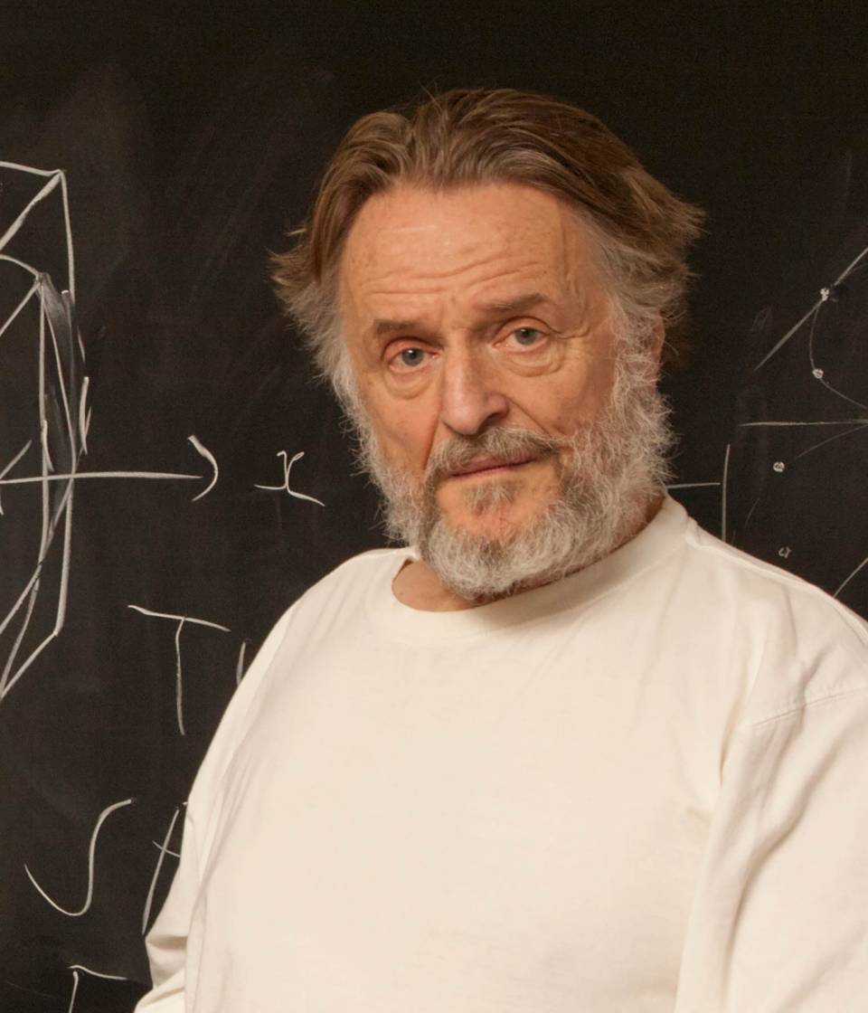
Figure: Left A Glider pattern discovered 1969 by Richard K. Guy. Right. John Horton Conway, creator of Life (1937-2020).

The glider was ‘discovered’ in 1969 by Richard K. Guy. What do we mean by discovered in this context? Well, as soon as the game of life is defined, objects such as the glider do somehow exist, but the many configurations of the game mean that it takes some time for us to see one and know it exists. This means, that despite being the creator, Conway, and despite the rules of the game being simple, and despite the rules being deterministic, we are not ‘omniscient’ in any simplistic sense. It requires computation to ‘discover’ what can exist in this universe once it’s been defined.

Another spaceship is known as the ‘loafer.’ It was ‘discovered’ in 2013 by Josh Ball. So despite the game having existed for over forty years, and the rules of the game being simple, there are emergent behaviours that are unknown.

Loafer (2013)

Figure: Left A Loafer pattern discovered by Josh Ball in 2013. Right. John Horton Conway, creator of Life (1937-2020).

Contrast this with our situation where in ‘real life’ we don’t know the simple rules of the game, the state space is larger, and emergent behaviours (hurricanes, earthquakes, volcanos, climate change) have direct consequences for our daily lives, and we understand why the process of ‘understanding’ the physical world is so difficult. We also see immediately how much easier we might expect the physical sciences to be than the social sciences, where the emergent behaviours are contingent on highly complex human interactions.

The Centrifugal Governor

[edit]

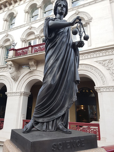
Figure: Centrifugal governor as held by “Science” on Holborn Viaduct

Boulton and Watt’s Steam Engine

[edit]

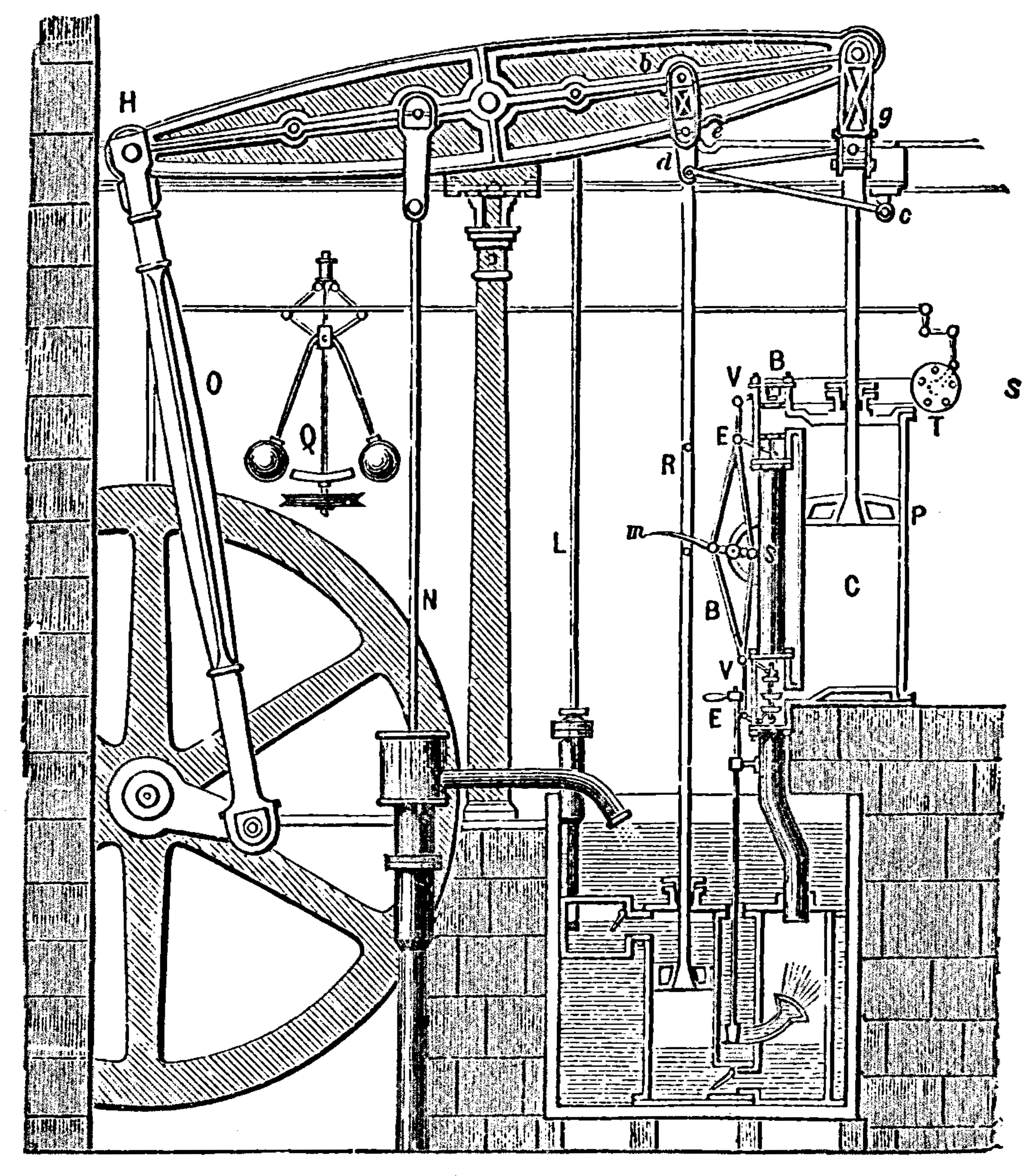
Figure: Watt’s Steam Engine which made Steam Power Efficient and Practical.

James Watt’s steam engine contained an early machine learning device. In the same way that modern systems are component based, his engine was composed of components. One of which is a speed regulator sometimes known as Watt’s governor. The two balls in the center of the image, when spun fast, rise, and through a linkage mechanism.

The centrifugal governor was made famous by Boulton and Watt when it was deployed in the steam engine. Studying stability in the governor is the main subject of James Clerk Maxwell’s paper on the theoretical analysis of governors (Maxwell, 1867). This paper is a founding paper of control theory. In an acknowledgment of its influence, Wiener used the name cybernetics to describe the field of control and communication in animals and the machine (Wiener, 1948). Cybernetics is the Greek word for governor, which comes from the latin for helmsman.

A governor is one of the simplest artificial intelligence systems. It senses the speed of an engine, and acts to change the position of the valve on the engine to slow it down.

Although it’s a mechanical system a governor can be seen as automating a role that a human would have traditionally played. It is an early example of artificial intelligence.

The centrifugal governor has several parameters, the weight of the balls used, the length of the linkages and the limits on the balls movement.

Two principle differences exist between the centrifugal governor and artificial intelligence systems of today.

The centrifugal governor is a physical system and it is an integral part of a wider physical system that it regulates (the engine).
The parameters of the governor were set by hand, our modern artificial intelligence systems have their parameters set by data.

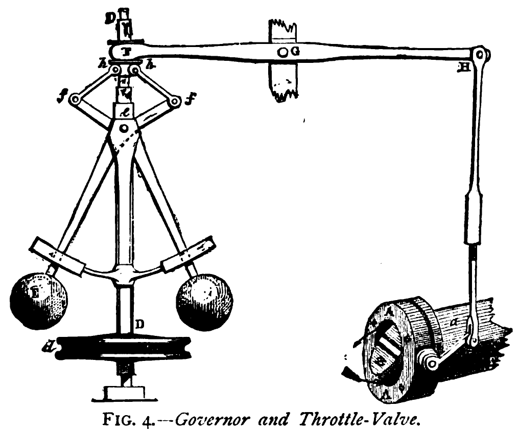
Figure: The centrifugal governor, an early example of a decision making system. The parameters of the governor include the lengths of the linkages (which effect how far the throttle opens in response to movement in the balls), the weight of the balls (which effects inertia) and the limits of to which the balls can rise.

This has the basic components of sense and act that we expect in an intelligent system, and this system saved the need for a human operator to manually adjust the system in the case of overspeed. Overspeed has the potential to destroy an engine, so the governor operates as a safety device.

The first wave of automation did bring about sabotoage as a worker’s response. But if machinery was sabotaged, for example, if the linkage between sensor (the spinning balls) and action (the valve closure) was broken, this would be obvious to the engine operator at start up time. The machine could be repaired before operation.

There is a gap between the world of data science and AI.
The mapping of the virtual onto the physical world.
E.g. Causal understanding.

Prime Air

[edit]

One project where a number of components of machine learning and the physical world come together is Amazon’s Prime Air drone delivery system.

Automating the process of moving physical goods through autonomous vehicles completes the loop between the ‘bits’ and the ‘atoms.’ In other words, the information and the ‘stuff.’ The idea of the drone is to complete a component of package delivery, the notion of last mile movement of goods, but in a fully autonomous way.

Figure: An actual Santa’s sleigh. Amazon’s new delivery drone. Machine learning algorithms are used across various systems including sensing (computer vision for detection of wires, people, dogs etc) and piloting. The technology is necessarily a combination of old and new ideas. The transition from vertical to horizontal flight is vital for efficiency and requires sophisticated machine learning to achieve.

As Jeff Wilke (CEO of Amazon Retail) announced in June 2019 the technology is ready, but still needs operationalisation including e.g. regulatory approval.

Figure: Jeff Wilke (CEO Amazon Consumer) announcing the new drone at the Amazon 2019 re:MARS event alongside the scale of the Amazon supply chain.

When we announced earlier this year that we were evolving our Prime two-day shipping offer in the U.S. to a one-day program, the response was terrific. But we know customers are always looking for something better, more convenient, and there may be times when one-day delivery may not be the right choice. Can we deliver packages to customers even faster? We think the answer is yes, and one way we’re pursuing that goal is by pioneering autonomous drone technology.

Today at Amazon’s re:MARS Conference (Machine Learning, Automation, Robotics and Space) in Las Vegas, we unveiled our latest Prime Air drone design. We’ve been hard at work building fully electric drones that can fly up to 15 miles and deliver packages under five pounds to customers in less than 30 minutes. And, with the help of our world-class fulfillment and delivery network, we expect to scale Prime Air both quickly and efficiently, delivering packages via drone to customers within months.

The 15 miles in less than 30 minutes implies air speed velocities of around 50 kilometers per hour.

Our newest drone design includes advances in efficiency, stability and, most importantly, in safety. It is also unique, and it advances the state of the art. How so? First, it’s a hybrid design. It can do vertical takeoffs and landings – like a helicopter. And it’s efficient and aerodynamic—like an airplane. It also easily transitions between these two modes—from vertical-mode to airplane mode, and back to vertical mode.

It’s fully shrouded for safety. The shrouds are also the wings, which makes it efficient in flight.

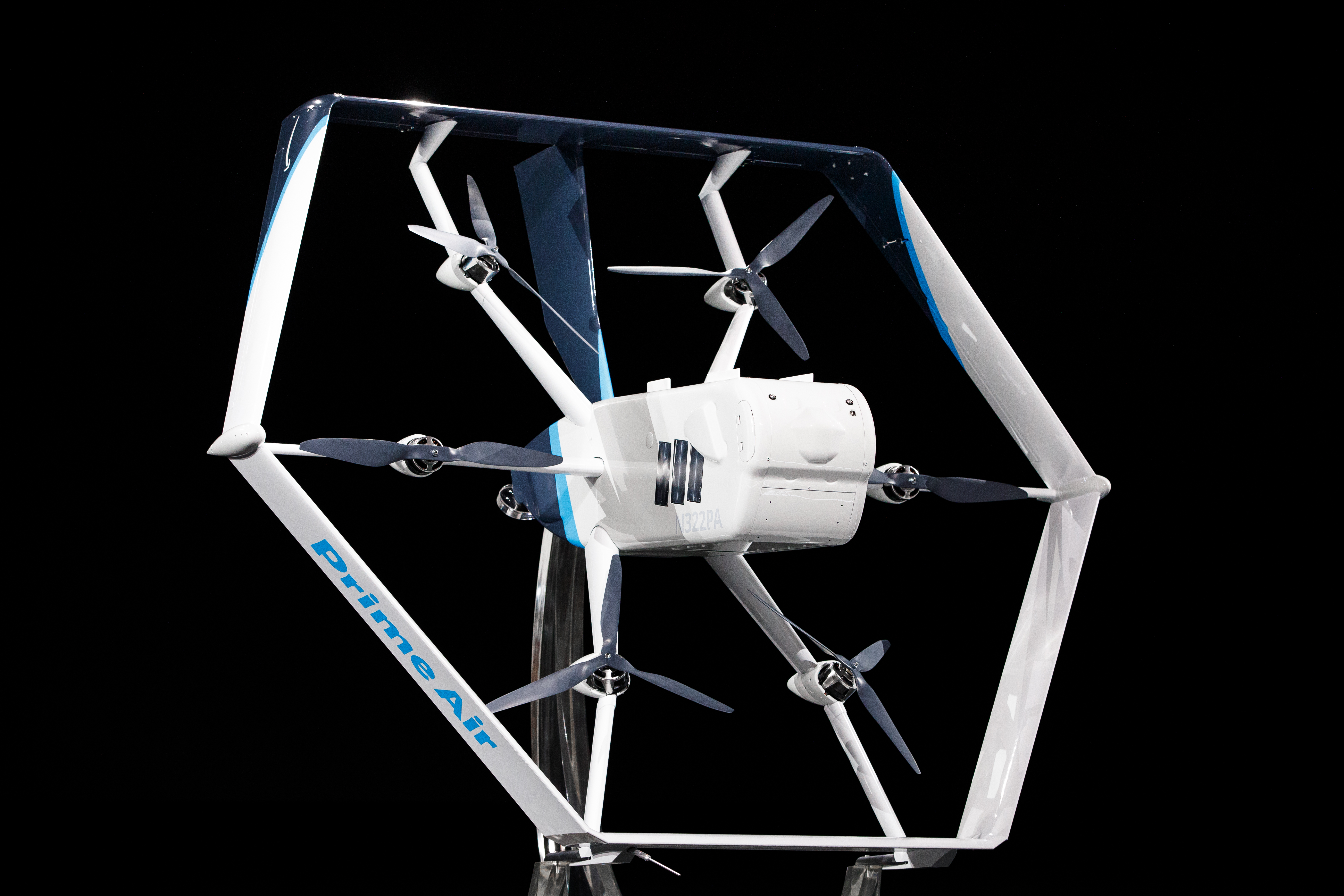
Figure: Picture of the drone from Amazon Re-MARS event in 2019.

Our drones need to be able to identify static and moving objects coming from any direction. We employ diverse sensors and advanced algorithms, such as multi-view stereo vision, to detect static objects like a chimney. To detect moving objects, like a paraglider or helicopter, we use proprietary computer-vision and machine learning algorithms.

A customer’s yard may have clotheslines, telephone wires, or electrical wires. Wire detection is one of the hardest challenges for low-altitude flights. Through the use of computer-vision techniques we’ve invented, our drones can recognize and avoid wires as they descend into, and ascend out of, a customer’s yard.

Buying System

[edit]

An example of a complex decision making system might be an automated buying system. In such a system, the idea is to match demand for products to supply of products.

The matching of demand and supply is a repetetive theme for decision making systems. Not only does it occur in automated buying, but also in the allocation of drivers to riders in a ride sharing system. Or in the allocation of compute resource to users in a cloud system.

The components of any of these system include: predictions of the demand for the product, or the drivers or the compute. Then predictions of the supply. Decisions are then made for how much material to keep in stock, or how many drivers to have on the road, or how much computer capacity to have in your data centres. These decisions have cost implications. The optimal amount of product will depend on the cost of making it available. For a buying system this is the storage costs.

Decisions are made on the basis of the supply and demand to make new orders, to encourage more drivers to come into the system or to build new data centers or rent more computational power.

Figure: The components of a putative automated buying system

Monolithic System

The classical approach to building these systems was a ‘monolithic system.’ Built in a similar way to the successful applicaitons software such as Excel or Word, or large operating systems, a single code base was constructed. The complexity of such code bases run to many lines.

In practice, shared dynamically linked libraries may be used for aspects such as user interface, or networking, but the software often has many millions of lines of code. For example, the Microsoft Office suite is said to contain over 30 millions of lines of code.

Figure: A potential path of models in a machine learning system.

Service Oriented Architecture

Such software is not only difficult to develop, it is difficult to scale when computation demands increase. Amazon’s original website software (called Obidos) was a monolithic design but by the early noughties it was becoming difficult to sustain and maintain. The software was phased out in 2006 to be replaced by a modularized software known as a ‘service oriented architecture.’

In Service Oriented Architecture, or “Software as a Service” the idea is that code bases are modularized and communicate with one another using network requests. A standard approach is to use a REST API. So, rather than a single monolithic code base, the code is developed with individual services that handle the different requests.

Figure: A potential path of models in a machine learning system.

This is the landscape we now find ourselves in with regard to software development. In practice, each of these services is often ‘owned’ and maintained by an individual team. The team is judged by the quality of their service provision. They work to detailed specifications on what their service should output, what its availability should be and other objectives like speed of response. This allows for conditional independence between teams and for faster development.

Intellectual Debt

[edit]

Figure: Jonathan Zittrain’s term to describe the challenges of explanation that come with AI is Intellectual Debt.

In computer systems the concept of technical debt has been surfaced by authors including Sculley et al. (2015). It is an important concept, that I think is somewhat hidden from the academic community, because it is a phenomenon that occurs when a computer software system is deployed.

Separation of Concerns

[edit]

To construct such complex systems an approach known as “separation of concerns” has been developed. The idea is that you architect your system, which consists of a large-scale complex task, into a set of simpler tasks. Each of these tasks is separately implemented. This is known as the decomposition of the task.

This is where Jonathan Zittrain’s beautifully named term “intellectual debt” rises to the fore. Separation of concerns enables the construction of a complex system. But who is concerned with the overall system?

Technical debt is the inability to maintain your complex software system.
Intellectual debt is the inability to explain your software system.

It is right there in our approach to software engineering. “Separation of concerns” means no one is concerned about the overall system itself.

Statistical Emulation

[edit]

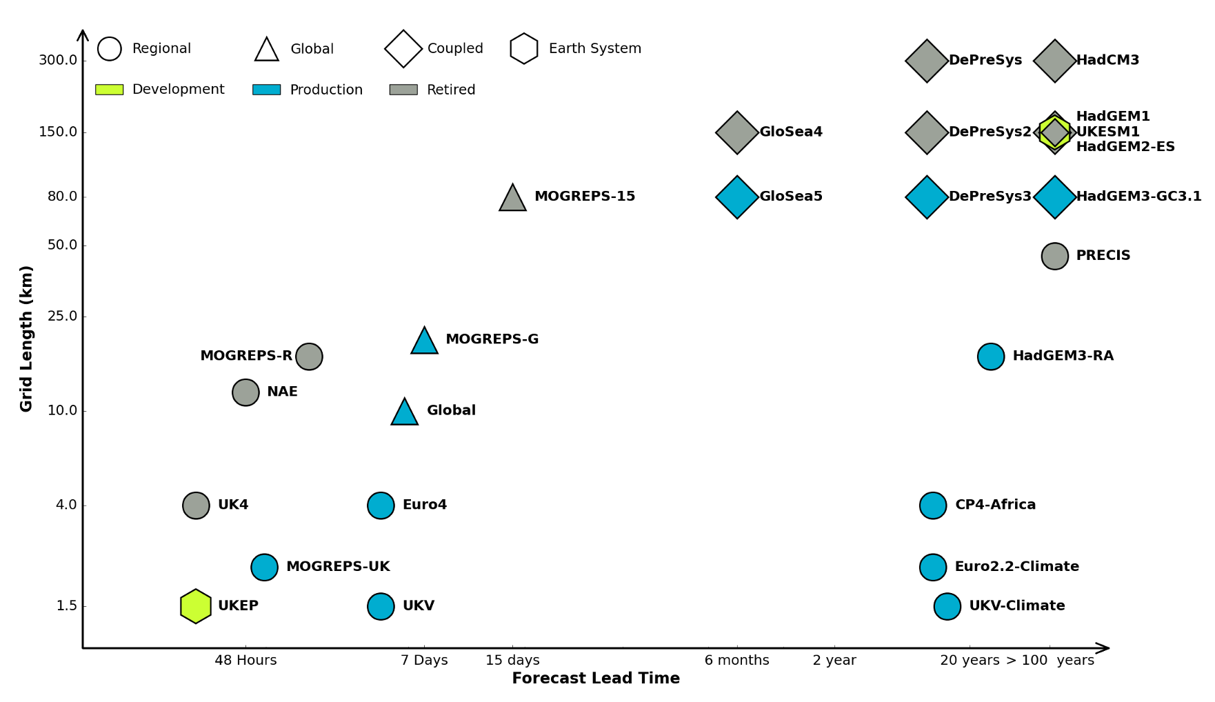
Figure: The UK Met office runs a shared code base for its simulations of climate and the weather. This plot shows the different spatial and temporal scales used.

In many real world systems, decisions are made through simulating the environment. Simulations may operate at different granularities. For example, simulations are used in weather forecasts and climate forecasts. Interestingly, the UK Met office uses the same code for both, it has a “Unified Model” approach, but they operate climate simulations one at greater spatial and temporal resolutions.

Figure: Real world systems consist of simulators that capture our domain knowledge about how our systems operate. Different simulators run at different speeds and granularities.

Figure: A statistical emulator is a system that reconstructs the simulation with a statistical model.

A statistical emulator is a data-driven model that learns about the underlying simulation. Importantly, learns with uncertainty, so it ‘knows what it doesn’t know.’ In practice, we can call the emulator in place of the simulator. If the emulator ‘doesn’t know,’ it can call the simulator for the answer.

Figure: A statistical emulator is a system that reconstructs the simulation with a statistical model. As well as reconstructing the simulation, a statistical emulator can be used to correlate with the real world.

As well as reconstructing an individual simulator, the emulator can calibrate the simulation to the real world, by monitoring differences between the simulator and real data. This allows the emulator to characterise where the simulation can be relied on, i.e. we can validate the simulator.

Similarly, the emulator can adjudicate between simulations. This is known as multi-fidelity emulation. The emulator characterizes which emulations perform well where.

If all this modelling is done with judiscious handling of the uncertainty, the computational doubt, then the emulator can assist in desciding what experiment should be run next to aid a decision: should we run a simulator, in which case which one, or should we attempt to acquire data from a real world intervention.

Auto AI

[edit]

Supervised machine learning models are data-driven statistical functional estimators. Each ML model is trained to perform a task. Machine learning systems are created when these models are integrated as interacting components in a more complex system that carries out a larger scale task, e.g. an autonomous drone delivery system.

Artificial Intelligence can also be seen as algorithmic decision-making. ML systems are data driven algorithmic decision-makers. Designing decision-making engines requires us to firstly decompose the system into its component parts. The decompositions are driven by (1) system performance requirements (2) the suite of ML algorithms at our disposal (3) the data availability. Performance requirements could be computational speed, accuracy, interpretability, and ‘fairness.’ The current generation of ML Systems is often based around supervised learning and human annotated data. But in the future, we may expect more use of reinforcement learning and automated knowledge discovery using unsupervised learning.

The classical systems approach assumes decomposability of components. In ML, upstream components (e.g. a pedestrian detector in an autonomous vehicle) make decisions that require revisiting once a fuller picture is realized at a downstream stage (e.g. vehicle path planning). The relative weaknesses and strengths of the different component parts need to be assessed when resolving conflicts.

In long-term planning, e.g. logistics and supply chain, a plan may be computed multiple times under different constraints as data evolves. In logistics, an initial plan for delivery may be computed when an item is viewed on a webpage. Webpage waiting-time constraints dominate the solution we choose. However, when an order is placed the time constraint may be relaxed and an accuracy constraint or a cost constraint may now dominate.

Such sub-systems will make inconsistent decisions, but we should monitor and control the extent of the inconsistency.

One solution to aid with both the lack of decomposability of the components and the inconsistency between components is end-to-end learning of the system. End-to-end learning is when we use ML techniques to fit parameters across the entire decision pipeline. We exploit gradient descent and automated differentiation software to achieve this. However, components in the system may themselves be running a simulation (e.g. a transport delivery-time simulation) or optimization (e.g. a linear program) as a subroutine. This limits the universality of automatic differentiation. Another alternative is to replace the entire system with a single ML model, such as in Deep Reinforcement Learning. However, this can severely limit the interpretability of the resulting system.

We envisage AutoAI as allowing us to take advantage of end-to-end learning without sacrificing the interpretability of the underlying system. Instead of optimizing each component individually, we introduce Bayesian system optimization (BSO). We will make use of the end-to-end learning signals and attribute them to the system sub-components through the construction of an interconnected network of surrogate models, known as emulators, each of which is associated with an individual component from the underlying ML-system. Instead of optimizing each component individually (e.g. by classical Bayesian optimization) in BSO we account for upstream and downstream interactions in the optimization, leveraging our end-to-end knowledge without damaging the interpretability of the underlying system.

Deep Emulation

[edit]

Figure: A potential path of models in a machine learning system.

As a solution we can use of emulators. When constructing an ML system, software engineers, ML engineers, economists and operations researchers are explicitly defining relationships between variables of interest in the system. That implicitly defines a joint distribution, $p(\mathbf{ y}^*, \mathbf{ y})$. In a decomposable system any sub-component may be defined as $p(\mathbf{ y}_\mathbf{i}|\mathbf{ y}_\mathbf{j})$ where $\mathbf{ y}_\mathbf{i}$ and $\mathbf{ y}_\mathbf{j}$ represent sub-sets of the full set of variables $\left\{\mathbf{ y}^*, \mathbf{ y}\right\}$. In those cases where the relationship is deterministic, the probability density would collapse to a vector-valued deterministic function, $\mathbf{ f}_\mathbf{i}\left(\mathbf{ y}_\mathbf{j}\right)$.

Inter-variable relationships could be defined by, for example a neural network (machine learning), an integer program (operational research), or a simulation (supply chain). This makes probabilistic inference in this joint density for real world systems is either very hard or impossible.

Emulation is a form of meta-modelling: we construct a model of the model. We can define the joint density of an emulator as $s(\mathbf{ y}*, \mathbf{ y})$, but if this probability density is to be an accurate representation of our system, it is likely to be prohibitively complex. Current practice is to design an emulator to deal with a specific question. This is done by fitting an ML model to a simulation from the the appropriate conditional distribution, $p(\mathbf{ y}_\mathbf{i}|\mathbf{ y}_\mathbf{j})$, which is intractable. The emulator provides an approximated answer of the form $s(\mathbf{ y}_\mathbf{i}|\mathbf{ y}_\mathbf{j})$. Critically, an emulator should incorporate its uncertainty about its approximation. So the emulator answer will be less certain than direct access to the conditional $p(\mathbf{ y}_i|\mathbf{ y}_j)$, but it may be sufficiently confident to act upon. Careful design of emulators to answer a given question leads to efficient diagnostics and understanding of the system. But in a complex interacting system an exponentially increasing number of questions can be asked. This calls for a system of automated construction of emulators which selects the right structure and redeploys the emulator as necessary. Rapid redeployment of emulators could exploit pre-existing emulators through transfer learning.

Automatically deploying these families of emulators for full system understanding is highly ambitious. It requires advances in engineering infrastructure, emulation and Bayesian optimization. However, the intermediate steps of developing this architecture also allow for automated monitoring of system accuracy and fairness. This facilitates AutoML on a component-wise basis which we can see as a simple implementation of AutoAI. The proposal is structured so that despite its technical ambition there is a smooth ramp of benefits to be derived across the programme of work.

In Applied Mathematics, the field studying these techniques is known as uncertainty quantification. The new challenge is the automation of emulator creation on demand to answer questions of interest and facilitate the system design, i.e. AutoAI through BSO.

At design stage, any particular AI task could be decomposed in multiple ways. Bayesian system optimization will assist both in determining the large-scale system design through exploring different decompositions and in refinement of the deployed system.

So far, most work on emulators has focussed on emulating a single component. Automated deployment and maintenance of ML systems requires networks of emulators that can be deployed and redeployed on demand depending on the particular question of interest. Therefore, the technical innovations we require are in the mathematical composition of emulator models (Damianou and Lawrence, 2013; Perdikaris et al., 2017). Different chains of emulators will need to be rapidly composed to make predictions of downstream performance. This requires rapid retraining of emulators and propagation of uncertainty through the emulation pipeline a process we call deep emulation.

Recomposing the ML system requires structural learning of the network. By parameterizing covariance functions appropriately this can be done through Gaussian processes (e.g. (Damianou et al., n.d.)), but one could also consider Bayesian neural networks and other generative models, e.g. Generative Adversarial Networks (Goodfellow et al., 2014).

Figure: A potential path of models in a machine learning system.

The Accelerate Programme

[edit]

Figure: The Accelerate Programme for Scientific Discovery covers research, education and training, engagement. Our aim is to bring about a step change in scientific discovery through AI. http://acceleratescience.github.io

We’re now in a new phase of the development of computing, with rapid advances in machine learning. But we see some of the same issues – researchers across disciplines hope to make use of machine learning, but need access to skills and tools to do so, while the field machine learning itself will need to develop new methods to tackle some complex, ‘real world’ problems.

It is with these challenges in mind that the Computer Lab has started the Accelerate Programme for Scientific Discovery. This new Programme is seeking to support researchers across the University to develop the skills they need to be able to use machine learning and AI in their research.

To do this, the Programme is developing three areas of activity:

Research: we’re developing a research agenda that develops and applies cutting edge machine learning methods to scientific challenges, with four Accelerate Research fellows working directly on issues relating to computational biology, psychiatry, string theory and materials science. While we’re concentrating on STEM subjects for now, in the longer term our ambition is to build links with the social sciences and humanities.
Teaching and learning: building on the teaching activities already delivered through University courses, we’re creating a pipeline of learning opportunities to help PhD students and postdocs better understand how to use data science and machine learning in their work. Our programme with Spark is one element of this, and we’ll be announcing further activities soon.
Engagement: we hope that Accelerate will help build a community of researchers working across the University at the interface on machine learning and the sciences, helping to share best practice and new methods, and support each other in advancing their research. Over the coming years, we’ll be running a variety of events and activities in support of this, and would welcome your ideas about what might be most useful.

ML and the Physical World Course

[edit]

Figure: Machine Learning and the Physical World is a course focussed on teaching the principles and techniques of emulation. It’s freely available on line. http://mlatcl.github.io/mlphysical/

The ML and the Physical World course is focused on machine learning systems that interact directly with the real world. Building artificial systems that interact with the physical world have significantly different challenges compared to the purely digital domain. In the real world data is scares, often uncertain and decisions can have costly and irreversible consequences. However, we also have the benefit of centuries of scientific knowledge that we can draw from. This module will provide the methodological background to machine learning applied in this scenario. We will study how we can build models with a principled treatment of uncertainty, allowing us to leverage prior knowledge and provide decisions that can be interrogated.

Thanks!

For more information on these subjects and more you might want to check the following resources.

References

Damianou, A., Ek, C.H., Titsias, M.K., Lawrence, N.D., n.d. Manifold relevance determination.

Damianou, A., Lawrence, N.D., 2013. Deep Gaussian processes. pp. 207–215.

Goodfellow, I., Pouget-Abadie, J., Mirza, M., Xu, B., Warde-Farley, D., Ozair, S., Courville, A., Bengio, Y., 2014. Generative adversarial nets, in: Ghahramani, Z., Welling, M., Cortes, C., Lawrence, N.D., Weinberger, K.Q. (Eds.), Advances in Neural Information Processing Systems 27. Curran Associates, Inc., pp. 2672–2680.

Maxwell, J.C., 1867. On governors. Proceedings of the Royal Society of London 16, 270–283.

Perdikaris, P., Raissi, M., Damianou, A., Lawrence, N.D., Karnidakis, G.E., 2017. Nonlinear information fusion algorithms for data-efficient multi-fidelity modelling. Proc. R. Soc. A 473. https://doi.org/10.1098/rspa.2016.0751

Sculley, D., Holt, G., Golovin, D., Davydov, E., Phillips, T., Ebner, D., Chaudhary, V., Young, M., Crespo, J.-F., Dennison, D., 2015. Hidden technical debt in machine learning systems, in: Cortes, C., Lawrence, N.D., Lee, D.D., Sugiyama, M., Garnett, R. (Eds.), Advances in Neural Information Processing Systems 28. Curran Associates, Inc., pp. 2503–2511.

Wiener, N., 1948. Cybernetics: Control and communication in the animal and the machine. MIT Press, Cambridge, MA.