The Atomic Human
Links
Abstract
A vital perspective is missing from the discussions we’re having about Artificial Intelligence: what does it mean for our identity?
Our fascination with AI stems from the perceived uniqueness of human intelligence. We believe it’s what differentiates us. Fears of AI not only concern how it invades our digital lives, but also the implied threat of an intelligence that displaces us from our position at the centre of the world.
Atomism, proposed by Democritus, suggested it was impossible to continue dividing matter down into ever smaller components: eventually we reach a point where a cut cannot be made (the Greek for uncuttable is ‘atom’). In the same way, by slicing away at the facets of human intelligence that can be replaced by machines, AI uncovers what is left: an indivisible core that is the essence of humanity.
By contrasting our own (evolved, locked-in, embodied) intelligence with the capabilities of machine intelligence through history, The Atomic Human reveals the technical origins, capabilities and limitations of AI systems, and how they should be wielded. Not just by the experts, but ordinary people. Either AI is a tool for us, or we become a tool of AI. Understanding this will enable us to choose the future we want.
This talk is based on Neil’s forthcoming book to be published with Allen Lane in June 2024. Machine learning solutions, in particular those based on deep learning methods, form an underpinning of the current revolution in “artificial intelligence” that has dominated popular press headlines and is having a significant influence on the wider tech agenda.
In this talk I will give an overview of where we are now with machine learning solutions, and what challenges we face both in the near and far future. These include practical application of existing algorithms in the face of the need to explain decision making, mechanisms for improving the quality and availability of data, dealing with large unstructured datasets.
The Atomic Human
Henry Ford’s Faster Horse


Figure: A 1925 Ford Model T built at Henry Ford’s Highland Park Plant in Dearborn, Michigan. This example now resides in Australia, owned by the founder of FordModelT.net. From https://commons.wikimedia.org/wiki/File:1925_Ford_Model_T_touring.jpg
It’s said that Henry Ford’s customers wanted a “a faster horse”. If Henry Ford was selling us artificial intelligence today, what would the customer call for, “a smarter human”? That’s certainly the picture of machine intelligence we find in science fiction narratives, but the reality of what we’ve developed is much more mundane.
Car engines produce prodigious power from petrol. Machine intelligences deliver decisions derived from data. In both cases the scale of consumption enables a speed of operation that is far beyond the capabilities of their natural counterparts. Unfettered energy consumption has consequences in the form of climate change. Does unbridled data consumption also have consequences for us?
If we devolve decision making to machines, we depend on those machines to accommodate our needs. If we don’t understand how those machines operate, we lose control over our destiny. Our mistake has been to see machine intelligence as a reflection of our intelligence. We cannot understand the smarter human without understanding the human. To understand the machine, we need to better understand ourselves.
Embodiment Factors
| bits/min | billions | 2,000 |
|
billion calculations/s |
~100 | a billion |
| embodiment | 20 minutes | 5 billion years |
Figure: Embodiment factors are the ratio between our ability to compute and our ability to communicate. Relative to the machine we are also locked in. In the table we represent embodiment as the length of time it would take to communicate one second’s worth of computation. For computers it is a matter of minutes, but for a human, it is a matter of thousands of millions of years. See also “Living Together: Mind and Machine Intelligence” Lawrence (2017)
There is a fundamental limit placed on our intelligence based on our ability to communicate. Claude Shannon founded the field of information theory. The clever part of this theory is it allows us to separate our measurement of information from what the information pertains to.1
Shannon measured information in bits. One bit of information is the amount of information I pass to you when I give you the result of a coin toss. Shannon was also interested in the amount of information in the English language. He estimated that on average a word in the English language contains 12 bits of information.
Given typical speaking rates, that gives us an estimate of our ability to communicate of around 100 bits per second (Reed and Durlach, 1998). Computers on the other hand can communicate much more rapidly. Current wired network speeds are around a billion bits per second, ten million times faster.
When it comes to compute though, our best estimates indicate our computers are slower. A typical modern computer can process make around 100 billion floating-point operations per second, each floating-point operation involves a 64 bit number. So the computer is processing around 6,400 billion bits per second.
It’s difficult to get similar estimates for humans, but by some estimates the amount of compute we would require to simulate a human brain is equivalent to that in the UK’s fastest computer (Ananthanarayanan et al., 2009), the MET office machine in Exeter, which in 2018 ranked as the 11th fastest computer in the world. That machine simulates the world’s weather each morning, and then simulates the world’s climate in the afternoon. It is a 16-petaflop machine, processing around 1,000 trillion bits per second.
Revolution
Arguably the information revolution we are experiencing is unprecedented in history. But changes in the way we share information have a long history. Over 5,000 years ago in the city of Uruk, on the banks of the Euphrates, communities which relied on the water to irrigate their corps developed an approach to recording transactions in clay. Eventually the system of recording system became sophisticated enough that their oral histories could be recorded in the form of the first epic: Gilgamesh.

Figure: Chicago Stone, side 2, recording sale of a number of fields, probably from Isin, Early Dynastic Period, c. 2600 BC, black basalt
It was initially develoepd for people as a recordd of who owed what to whom, expanding individuals’ capacity to remember. But over a five hundred year period writing evolved to become a tool for literature as well. More pithily put, writing was invented by accountants not poets (see e.g. this piece by Tim Harford).
In some respects today’s revolution is different, because it involves also the creation of stories as well as their curation. But in some fundamental ways we can see what we have produced as another tool for us in the information revolution.
Information and Embodiment
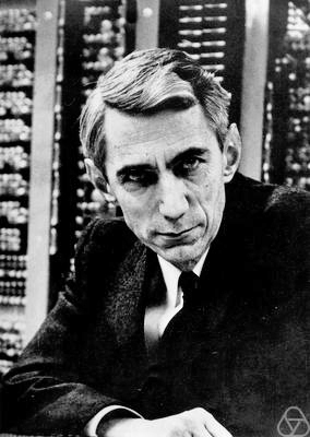
Figure: Claude Shannon (1916-2001)
| bits/min | billions | 2,000 |
|
billion calculations/s |
~100 | a billion |
| embodiment | 20 minutes | 5 billion years |
Figure: Embodiment factors are the ratio between our ability to compute and our ability to communicate. Relative to the machine we are also locked in. In the table we represent embodiment as the length of time it would take to communicate one second’s worth of computation. For computers it is a matter of minutes, but for a human, it is a matter of thousands of millions of years.
New Flow of Information
Classically the field of statistics focused on mediating the relationship between the machine and the human. Our limited bandwidth of communication means we tend to over-interpret the limited information that we are given, in the extreme we assign motives and desires to inanimate objects (a process known as anthropomorphizing). Much of mathematical statistics was developed to help temper this tendency and understand when we are valid in drawing conclusions from data.
Figure: The trinity of human, data, and computer, and highlights the modern phenomenon. The communication channel between computer and data now has an extremely high bandwidth. The channel between human and computer and the channel between data and human is narrow. New direction of information flow, information is reaching us mediated by the computer. The focus on classical statistics reflected the importance of the direct communication between human and data. The modern challenges of data science emerge when that relationship is being mediated by the machine.
Data science brings new challenges. In particular, there is a very large bandwidth connection between the machine and data. This means that our relationship with data is now commonly being mediated by the machine. Whether this is in the acquisition of new data, which now happens by happenstance rather than with purpose, or the interpretation of that data where we are increasingly relying on machines to summarize what the data contains. This is leading to the emerging field of data science, which must not only deal with the same challenges that mathematical statistics faced in tempering our tendency to over interpret data but must also deal with the possibility that the machine has either inadvertently or maliciously misrepresented the underlying data.
Societal Effects
We have already seen the effects of this changed dynamic in biology and computational biology. Improved sensorics have led to the new domains of transcriptomics, epigenomics, and ‘rich phenomics’ as well as considerably augmenting our capabilities in genomics.
Biologists have had to become data-savvy, they require a rich understanding of the available data resources and need to assimilate existing data sets in their hypothesis generation as well as their experimental design. Modern biology has become a far more quantitative science, but the quantitativeness has required new methods developed in the domains of computational biology and bioinformatics.
There is also great promise for personalized health, but in health the wide data-sharing that has underpinned success in the computational biology community is much harder to carry out.
We can expect to see these phenomena reflected in wider society. Particularly as we make use of more automated decision making based only on data. This is leading to a requirement to better understand our own subjective biases to ensure that the human to computer interface allows domain experts to assimilate data driven conclusions in a well calibrated manner. This is particularly important where medical treatments are being prescribed. It also offers potential for different kinds of medical intervention. More subtle interventions are possible when the digital environment is able to respond to users in an bespoke manner. This has particular implications for treatment of mental health conditions.
The main phenomenon we see across the board is the shift in dynamic from the direct pathway between human and data, as traditionally mediated by classical statistics, to a new flow of information via the computer. This change of dynamics gives us the modern and emerging domain of data science, where the interactions between human and data are mediated by the machine.
The Great AI Fallacy
There is a lot of variation in the use of the term artificial intelligence. I’m sometimes asked to define it, but depending on whether you’re speaking to a member of the public, a fellow machine learning researcher, or someone from the business community, the sense of the term differs.
However, underlying its use I’ve detected one disturbing trend. A trend I’m beginining to think of as “The Great AI Fallacy”.
The fallacy is associated with an implicit promise that is embedded in many statements about Artificial Intelligence. Artificial Intelligence, as it currently exists, is merely a form of automated decision making. The implicit promise of Artificial Intelligence is that it will be the first wave of automation where the machine adapts to the human, rather than the human adapting to the machine.
How else can we explain the suspension of sensible business judgment that is accompanying the hype surrounding AI?
This fallacy is particularly pernicious because there are serious benefits to society in deploying this new wave of data-driven automated decision making. But the AI Fallacy is causing us to suspend our calibrated skepticism that is needed to deploy these systems safely and efficiently.
The problem is compounded because many of the techniques that we’re speaking of were originally developed in academic laboratories in isolation from real-world deployment.
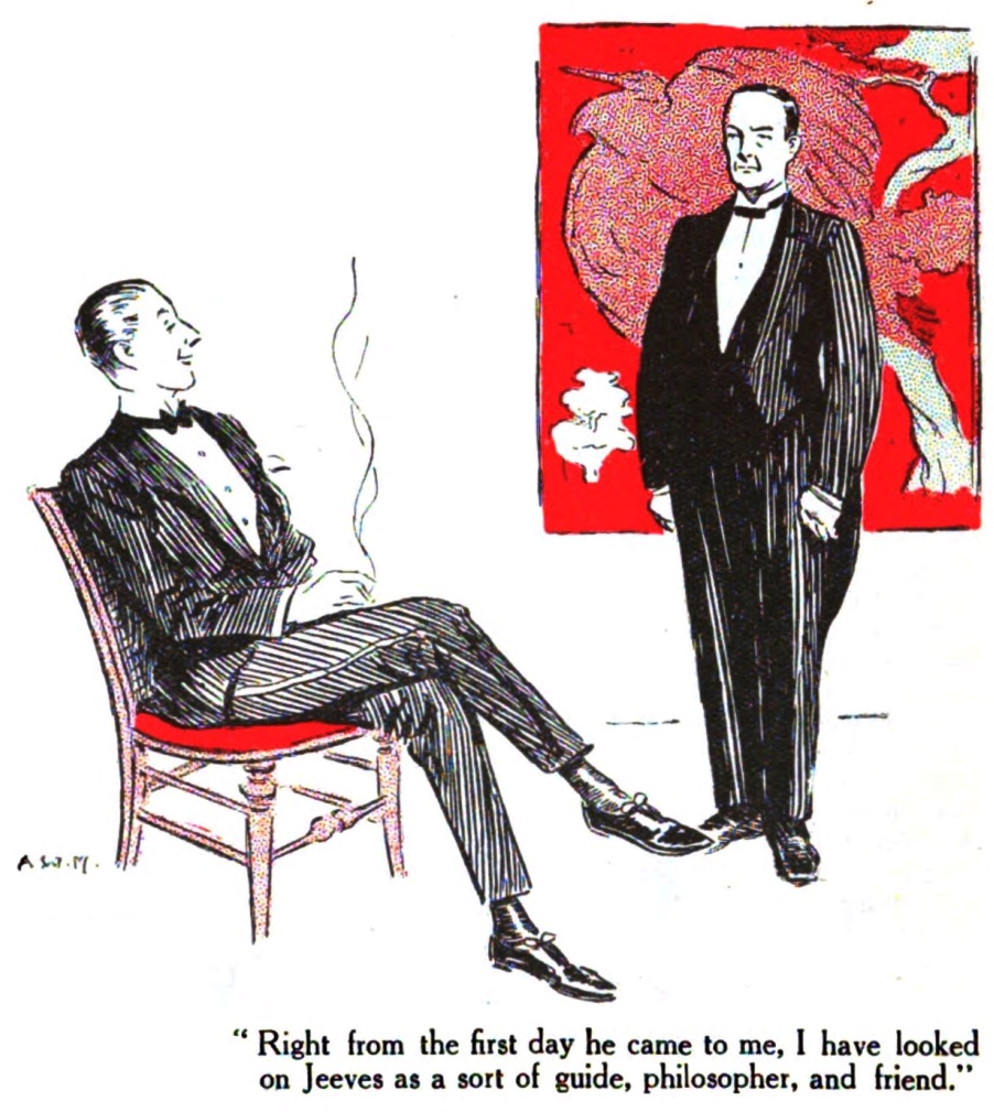
Figure: We seem to have fallen for a perspective on AI that suggests it will adapt to our schedule, rather in the manner of a 1930s manservant.
Lies and Damned Lies
There are three types of lies: lies, damned lies and statistics
Arthur Balfour 1848-1930
Arthur Balfour was quoting the lawyer James Munro2 when he said that there three types of lies: lies, damned lies and statistics in 1892. This is 20 years before the first academic department of applied statistics was founded at UCL. If Balfour were alive today, it is likely that he’d rephrase his quote:
There are three types of lies, lies damned lies and big data.
Why? Because the challenges of understanding and interpreting big data today are similar to those that Balfour (who was a Conservative politician and statesman and would later become Prime Minister) faced in governing an empire through statistics in the latter part of the 19th century.
The quote lies, damned lies and statistics was also credited to Benjamin Disraeli by Mark Twain in Twain’s autobiography.3 It characterizes the idea that statistic can be made to prove anything. But Disraeli died in 1881 and Mark Twain died in 1910. The important breakthrough in overcoming our tendency to over-interpet data came with the formalization of the field through the development of mathematical statistics.
Data has an elusive quality, it promises so much but can deliver little, it can mislead and misrepresent. To harness it, it must be tamed. In Balfour and Disraeli’s time during the second half of the 19th century, numbers and data were being accumulated, the social sciences were being developed. There was a large-scale collection of data for the purposes of government.
The modern ‘big data era’ is on the verge of delivering the same sense of frustration that Balfour experienced, the early promise of big data as a panacea is evolving to demands for delivery. For me, personally, peak-hype coincided with an email I received inviting collaboration on a project to deploy “Big Data and Internet of Things in an Industry 4.0 environment”. Further questioning revealed that the actual project was optimization of the efficiency of a manufacturing production line, a far more tangible and realizable goal.
The antidote to this verbiage is found in increasing awareness. When dealing with data the first trap to avoid is the games of buzzword bingo that we are wont to play. The first goal is to quantify what challenges can be addressed and what techniques are required. Behind the hype fundamentals are changing. The phenomenon is about the increasing access we have to data. The way customers’ information is recorded and processes are codified and digitized with little overhead. Internet of things is about the increasing number of cheap sensors that can be easily interconnected through our modern network structures. But businesses are about making money, and these phenomena need to be recast in those terms before their value can be realized.
For more thoughts on the challenges that statistics brings see Chapter 8 of Lawrence (2024).
Mathematical Statistics
Karl Pearson (1857-1936), Ronald Fisher (1890-1962) and others considered the question of what conclusions can truly be drawn from data. Their mathematical studies act as a restraint on our tendency to over-interpret and see patterns where there are none. They introduced concepts such as randomized control trials that form a mainstay of our decision making today, from government, to clinicians to large scale A/B testing that determines the nature of the web interfaces we interact with on social media and shopping.
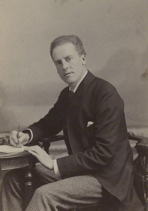
Figure: Karl Pearson (1857-1936), one of the founders of Mathematical Statistics.
Their movement did the most to put statistics to rights, to eradicate the ‘damned lies’. It was known as ‘mathematical statistics’. Today I believe we should look to the emerging field of data science to provide the same role. Data science is an amalgam of statistics, data mining, computer systems, databases, computation, machine learning and artificial intelligence. Spread across these fields are the tools we need to realize data’s potential. For many businesses this might be thought of as the challenge of ‘converting bits into atoms’. Bits: the data stored on computer, atoms: the physical manifestation of what we do; the transfer of goods, the delivery of service. From fungible to tangible. When solving a challenge through data there are a series of obstacles that need to be addressed.
Firstly, data awareness: what data you have and where its stored. Sometimes this includes changing your conception of what data is and how it can be obtained. From automated production lines to apps on employee smart phones. Often data is locked away: manual logbooks, confidential data, personal data. For increasing awareness an internal audit can help. The website data.gov.uk hosts data made available by the UK government. To create this website the government’s departments went through an audit of what data they each hold and what data they could make available. Similarly, within private businesses this type of audit could be useful for understanding their internal digital landscape: after all the key to any successful campaign is a good map.
Secondly, availability. How well are the data sources interconnected? How well curated are they? The curse of Disraeli was associated with unreliable data and unreliable statistics. The misrepresentations this leads to are worse than the absence of data as they give a false sense of confidence to decision making. Understanding how to avoid these pitfalls involves an improved sense of data and its value, one that needs to permeate the organization.
The final challenge is analysis, the accumulation of the necessary expertise to digest what the data tells us. Data requires interpretation, and interpretation requires experience. Analysis is providing a bottleneck due to a skill shortage, a skill shortage made more acute by the fact that, ideally, analysis should be carried out by individuals not only skilled in data science but also equipped with the domain knowledge to understand the implications in a given application, and to see opportunities for improvements in efficiency.
‘Mathematical Data Science’
As a term ‘big data’ promises much and delivers little, to get true value from data, it needs to be curated and evaluated. The three stages of awareness, availability and analysis provide a broad framework through which organizations should be assessing the potential in the data they hold. Hand waving about big data solutions will not do, it will only lead to self-deception. The castles we build on our data landscapes must be based on firm foundations, process and scientific analysis. If we do things right, those are the foundations that will be provided by the new field of data science.
Today the statement “There are three types of lies: lies, damned lies and ‘big data’” may be more apt. We are revisiting many of the mistakes made in interpreting data from the 19th century. Big data is laid down by happenstance, rather than actively collected with a particular question in mind. That means it needs to be treated with care when conclusions are being drawn. For data science to succeed it needs the same form of rigor that Pearson and Fisher brought to statistics, a “mathematical data science” is needed.
You can also check my blog post on Lies, Damned Lies and Big Data.
Human Communication
For human conversation to work, we require an internal model of who we are speaking to. We model each other, and combine our sense of who they are, who they think we are, and what has been said. This is our approach to dealing with the limited bandwidth connection we have. Empathy and understanding of intent. Mental dispositional concepts are used to augment our limited communication bandwidth.
Fritz Heider referred to the important point of a conversation as being that they are happenings that are “psychologically represented in each of the participants” (his emphasis) (Heider, 1958).
Bandwidth Constrained Conversations
Figure: Conversation relies on internal models of other individuals.
Figure: Misunderstanding of context and who we are talking to leads to arguments.
Embodiment factors imply that, in our communication between humans, what is not said is, perhaps, more important than what is said. To communicate with each other we need to have a model of who each of us are.
To aid this, in society, we are required to perform roles. Whether as a parent, a teacher, an employee or a boss. Each of these roles requires that we conform to certain standards of behaviour to facilitate communication between ourselves.
Control of self is vitally important to these communications.
The high availability of data available to humans undermines human-to-human communication channels by providing new routes to undermining our control of self.
Heider and Simmel (1944)
Figure: Fritz Heider and Marianne Simmel’s video of shapes from Heider and Simmel (1944).
Fritz Heider and Marianne Simmel’s experiments with animated shapes from 1944 (Heider and Simmel, 1944). Our interpretation of these objects as showing motives and even emotion is a combination of our desire for narrative, a need for understanding of each other, and our ability to empathize. At one level, these are crudely drawn objects, but in another way, the animator has communicated a story through simple facets such as their relative motions, their sizes and their actions. We apply our psychological representations to these faceless shapes to interpret their actions.
See also a recent review paper on Human Cooperation by Henrich and Muthukrishna (2021).
A Six Word Novel

Figure: Consider the six-word novel, apocryphally credited to Ernest Hemingway, “For sale: baby shoes, never worn”. To understand what that means to a human, you need a great deal of additional context. Context that is not directly accessible to a machine that has not got both the evolved and contextual understanding of our own condition to realize both the implication of the advert and what that implication means emotionally to the previous owner.
But this is a very different kind of intelligence than ours. A computer cannot understand the depth of the Ernest Hemingway’s apocryphal six-word novel: “For Sale, Baby Shoes, Never worn”, because it isn’t equipped with that ability to model the complexity of humanity that underlies that statement.
Computer Conversations
Figure: Conversation relies on internal models of other individuals.
Figure: Misunderstanding of context and who we are talking to leads to arguments.
Similarly, we find it difficult to comprehend how computers are making decisions. Because they do so with more data than we can possibly imagine.
In many respects, this is not a problem, it’s a good thing. Computers and us are good at different things. But when we interact with a computer, when it acts in a different way to us, we need to remember why.
Just as the first step to getting along with other humans is understanding other humans, so it needs to be with getting along with our computers.
Embodiment factors explain why, at the same time, computers are so impressive in simulating our weather, but so poor at predicting our moods. Our complexity is greater than that of our weather, and each of us is tuned to read and respond to one another.
Their intelligence is different. It is based on very large quantities of data that we cannot absorb. Our computers don’t have a complex internal model of who we are. They don’t understand the human condition. They are not tuned to respond to us as we are to each other.
Embodiment factors encapsulate a profound thing about the nature of humans. Our locked in intelligence means that we are striving to communicate, so we put a lot of thought into what we’re communicating with. And if we’re communicating with something complex, we naturally anthropomorphize them.
We give our dogs, our cats, and our cars human motivations. We do the same with our computers. We anthropomorphize them. We assume that they have the same objectives as us and the same constraints. They don’t.
This means, that when we worry about artificial intelligence, we worry about the wrong things. We fear computers that behave like more powerful versions of ourselves that will struggle to outcompete us.
In reality, the challenge is that our computers cannot be human enough. They cannot understand us with the depth we understand one another. They drop below our cognitive radar and operate outside our mental models.
The real danger is that computers don’t anthropomorphize. They’ll make decisions in isolation from us without our supervision because they can’t communicate truly and deeply with us.
Probability Conversations
Figure: The focus so far has been on reducing uncertainty to a few representative values and sharing numbers with human beings. We forget that most people can be confused by basic probabilities for example the prosecutor’s fallacy.
In practice we know that probabilities can be very unintuitive, for example in court there is a fallacy known as the “prosecutor’s fallacy” that confuses conditional probabilities. This can cause problems in jury trials (Thompson, 1989).
Networked Interactions
Our modern society intertwines the machine with human interactions. The key question is who has control over these interfaces between humans and machines.
Figure: Humans and computers interacting should be a major focus of our research and engineering efforts.
So the real challenge that we face for society is understanding which systemic interventions will encourage the right interactions between the humans and the machine at all of these interfaces.
Figure: Humans use culture, facts and ‘artefacts’ to communicate.
Number Theatre
Unfortunately, we don’t always have time to wait for this process to converge to an answer we can all rely on before a decision is required.
Not only can we be misled by data before a decision is made, but sometimes we can be misled by data to justify the making of a decision. David Spiegelhalter refers to the phenomenon of “Number Theatre” in a conversation with Andrew Marr from May 2020 on the presentation of data.
Figure: Professor Sir David Spiegelhalter on Andrew Marr on 10th May 2020 speaking about some of the challengers around data, data presentation, and decision making in a pandemic. David mentions number theatre at 9 minutes 10 seconds.
Data Theatre
Data Theatre exploits data inattention bias to present a particular view on events that may misrepresents through selective presentation. Statisticians are one of the few groups that are trained with a sufficient degree of data skepticism. But it can also be combatted through ensuring there are domain experts present, and that they can speak freely.
Figure: The phenomenon of number theatre or data theatre was described by David Spiegelhalter and is nicely summarized by Martin Robbins in this sub-stack article https://martinrobbins.substack.com/p/data-theatre-why-the-digital-dashboards.
LLM Conversations
Figure: The focus so far has been on reducing uncertainty to a few representative values and sharing numbers with human beings. We forget that most people can be confused by basic probabilities for example the prosecutor’s fallacy.
Figure: The Inner Monologue paper suggests using LLMs for robotic planning (Huang et al., 2023).
By interacting directly with machines that have an understanding of human cultural context, it should be possible to share the nature of uncertainty in the same way humans do. See for example the paper Inner Monologue: Embodied Reasoning through Planning Huang et al. (2023).
The MONIAC
The MONIAC was an analogue computer designed to simulate the UK economy. Analogue comptuers work through analogy, the analogy in the MONIAC is that both money and water flow. The MONIAC exploits this through a system of tanks, pipes, valves and floats that represent the flow of money through the UK economy. Water flowed from the treasury tank at the top of the model to other tanks representing government spending, such as health and education. The machine was initially designed for teaching support but was also found to be a useful economic simulator. Several were built and today you can see the original at Leeds Business School, there is also one in the London Science Museum and one in the Unisversity of Cambridge’s economics faculty.
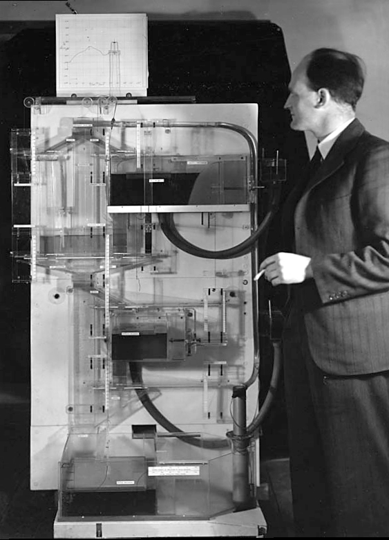
Figure: Bill Phillips and his MONIAC (completed in 1949). The machine is an analogue computer designed to simulate the workings of the UK economy.
Donald MacKay
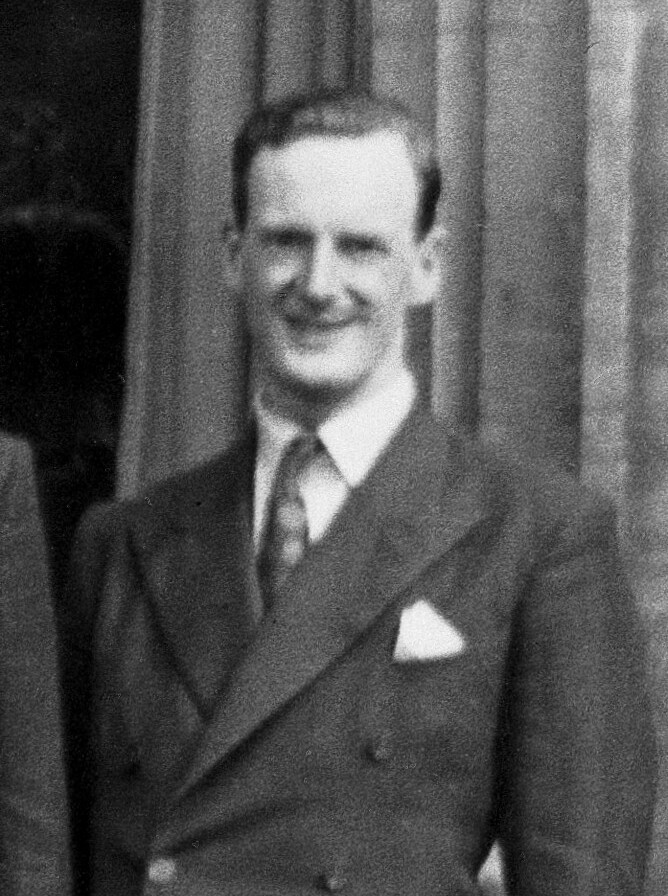
Figure: Donald M. MacKay (1922-1987), a physicist who was an early member of the cybernetics community and member of the Ratio Club.
Donald MacKay was a physicist who worked on naval gun targetting during the second world war. The challenge with gun targetting for ships is that both the target and the gun platform are moving. The challenge was tackled using analogue computers, for example in the US the Mark I fire control computer which was a mechanical computer. MacKay worked on radar systems for gun laying, here the velocity and distance of the target could be assessed through radar and an mechanical electrical analogue computer.
Fire Control Systems
Naval gunnery systems deal with targeting guns while taking into account movement of ships. The Royal Navy’s Gunnery Pocket Book (The Admiralty, 1945) gives details of one system for gun laying.
Like many challenges we face today, in the second world war, fire control was handled by a hybrid system of humans and computers. This means deploying human beings for the tasks that they can manage, and machines for the tasks that are better performed by a machine. This leads to a division of labour between the machine and the human that can still be found in our modern digital ecosystems.
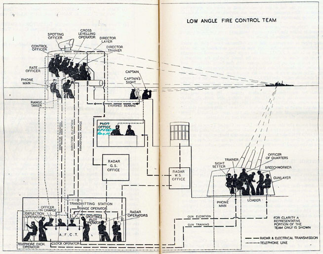
Figure: The fire control computer set at the centre of a system of observation and tracking (The Admiralty, 1945).
As analogue computers, fire control computers from the second world war would contain components that directly represented the different variables that were important in the problem to be solved, such as the inclination between two ships.

Figure: Measuring inclination between two ships (The Admiralty, 1945). Sophisticated fire control computers allowed the ship to continue to fire while under maneuvers.
The fire control systems were electro-mechanical analogue computers that represented the “state variables” of interest, such as inclination and ship speed with gears and cams within the machine.
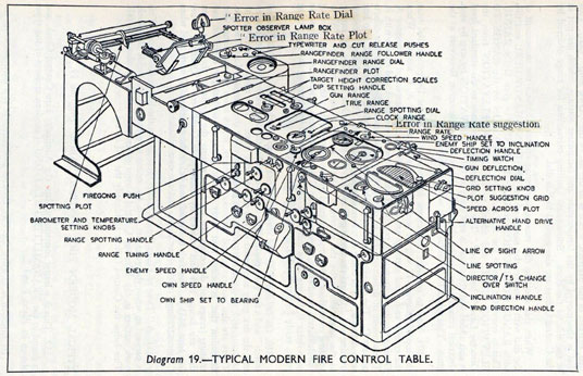
Figure: A second world war gun computer’s control table (The Admiralty, 1945).
For more details on fire control computers, you can watch a 1953 film on the the US the Mark IA fire control computer from Periscope Film.
Behind the Eye

Figure: Behind the Eye (MacKay, 1991) summarises MacKay’s Gifford Lectures, where MacKay uses the operation of the eye as a window on the operation of the brain.
Donald MacKay was at King’s College for his PhD. He was just down the road from Bill Phillips at LSE who was building the MONIAC. He was part of the Ratio Club. A group of early career scientists who were interested in communication and control in animals and humans, or more specifically they were interested in computers and brains. The were part of an international movement known as cybernetics.
Donald MacKay wrote of the influence that his own work on radar had on his interest in the brain.
… during the war I had worked on the theory of automated and electronic computing and on the theory of information, all of which are highly relevant to such things as automatic pilots and automatic gun direction. I found myself grappling with problems in the design of artificial sense organs for naval gun-directors and with the principles on which electronic circuits could be used to simulate situations in the external world so as to provide goal-directed guidance for ships, aircraft, missiles and the like.
Later in the 1940’s, when I was doing my Ph.D. work, there was much talk of the brain as a computer and of the early digital computers that were just making the headlines as “electronic brains.” As an analogue computer man I felt strongly convinced that the brain, whatever it was, was not a digital computer. I didn’t think it was an analogue computer either in the conventional sense.
But this naturally rubbed under my skin the question: well, if it is not either of these, what kind of system is it? Is there any way of following through the kind of analysis that is appropriate to their artificial automata so as to understand better the kind of system the human brain is? That was the beginning of my slippery slope into brain research.
Behind the Eye pg 40. Edited version of the 1986 Gifford Lectures given by Donald M. MacKay and edited by Valerie MacKay
Importantly, MacKay distinguishes between the analogue computer and the digital computer. As he mentions, his experience was with analogue machines. An analogue machine is literally an analogue. The radar systems that Wiener and MacKay both worked on were made up of electronic components such as resistors, capacitors, inductors and/or mechanical components such as cams and gears. Together these components could represent a physical system, such as an anti-aircraft gun and a plane. The design of the analogue computer required the engineer to simulate the real world in analogue electronics, using dualities that exist between e.g. mechanical circuits (mass, spring, damper) and electronic circuits (inductor, resistor, capacitor). The analogy between mass and a damper, between spring and a resistor and between capacitor and a damper works because the underlying mathematics is approximated with the same linear system: a second order differential equation. This mathematical analogy allowed the designer to map from the real world, through mathematics, to a virtual world where the components reflected the real world through analogy.
Human Analogue Machine
The machine learning systems we have built today that can reconstruct human text, or human classification of images, necessarily must have some aspects to them that are analagous to our understanding. As MacKay suggests the brain is neither a digital or an analogue computer, and the same can be said of the modern neural network systems that are being tagged as “artificial intelligence”.
I believe a better term for them is “human-analogue machines”, because what we have built is not a system that can make intelligent decisions from first principles (a rational approach) but one that observes how humans have made decisions through our data and reconstructs that process. Machine learning is more empiricist than rational, but now we n empirical approach that distils our evolved intelligence.

Figure: The human analogue machine creates a feature space which is analagous to that we use to reason, one way of doing this is to have a machine attempt to compress all human generated text in an auto-regressive manner.
The perils of developing this capability include counterfeit people, a notion that the philosopher Daniel Dennett has described in The Atlantic. This is where computers can represent themselves as human and fool people into doing things on that basis.
Intellectual Debt
Figure: Jonathan Zittrain’s term to describe the challenges of explanation that come with AI is Intellectual Debt.
In the context of machine learning and complex systems, Jonathan Zittrain has coined the term “Intellectual Debt” to describe the challenge of understanding what you’ve created. In the ML@CL group we’ve been foucssing on developing the notion of a data-oriented architecture to deal with intellectual debt (Cabrera et al., 2023).
Zittrain points out the challenge around the lack of interpretability of individual ML models as the origin of intellectual debt. In machine learning I refer to work in this area as fairness, interpretability and transparency or FIT models. To an extent I agree with Zittrain, but if we understand the context and purpose of the decision making, I believe this is readily put right by the correct monitoring and retraining regime around the model. A concept I refer to as “progression testing”. Indeed, the best teams do this at the moment, and their failure to do it feels more of a matter of technical debt rather than intellectual, because arguably it is a maintenance task rather than an explanation task. After all, we have good statistical tools for interpreting individual models and decisions when we have the context. We can linearise around the operating point, we can perform counterfactual tests on the model. We can build empirical validation sets that explore fairness or accuracy of the model.
But if we can avoid the pitfalls of counterfeit people, this also offers us an opportunity to psychologically represent (Heider, 1958) the machine in a manner where humans can communicate without special training. This in turn offers the opportunity to overcome the challenge of intellectual debt.
Despite the lack of interpretability of machine learning models, they allow us access to what the machine is doing in a way that bypasses many of the traditional techniques developed in statistics. But understanding this new route for access is a major new challenge.
Figure: The trinity of human, data, and computer, and highlights the modern phenomenon. The communication channel between computer and data now has an extremely high bandwidth. The channel between human and computer and the channel between data and human is narrow. New direction of information flow, information is reaching us mediated by the computer. The focus on classical statistics reflected the importance of the direct communication between human and data. The modern challenges of data science emerge when that relationship is being mediated by the machine.
Figure: The HAM now sits between us and the traditional digital computer.
Richard Feynmann on Doubt
One thing is I can live with is doubt, and uncertainty and not knowing. I think it’s much more interesting to live with not knowing than to have an answer that might be wrong.
Richard P. Feynmann in the The Pleasure of Finding Things Out 1981.
Conclusions
The probabilistic modelling community has evolved in an era where the assumption was that ambiguous conclusions are best shared with a (trained) professional through probabilities. Recent advances in generative AI offer the possibility of machines that have a better understanding of human subjective ambiguities and therefore machines that can summarise information in a way that can be interogated rather than just through a series of numbers.
Thanks!
For more information on these subjects and more you might want to check the following resources.
- twitter: @lawrennd
- podcast: The Talking Machines
- newspaper: Guardian Profile Page
- blog: http://inverseprobability.com