Abstract

In 2014, along with Corinna Cortes, I was Program Chair of the Neural Information Processing Systems conference. At the time, when wondering about innovations for the conference, Corinna and I decided it would be interesting to test the consistency of reviewing. With this in mind, we randomly selected 10% of submissions and had them reviewed by two independent committees. In this talk I will review the construction of the experiment, explain how the NeurIPS review process worked and talk about what I felt the implications for reviewing were, vs what the community reaction was.

Introduction

The NIPS experiment was an experiment to determine the consistency of the review process. After receiving papers, we selected 10% that would be independently rereviewed. The idea was to determine how consistent the decisions between the two sets of independent papers would be. In 2014 NIPS received 1678 submissions and we selected 170 for the experiment. These papers are referred to below as ‘duplicated papers.’

To run the experiment, we created two separate committees within the NIPS program committee. The idea was that the two separate committees would review each duplicated paper independently and results compared.

NeurIPS in Numbers

In 2014 the NeurIPS conference had 1474 active reviewers (up from 1133 in 2013), 92 area chairs (up from 67 in 2013) and two program chairs, Corinna Cortes and me.

The conference received 1678 submissions and presented 414 accepted papers, of which 20 were presented as talks in the single-track session, 62 were presented as spotlights and 331 papers were presented as posters. Of the 1678 submissions, 19 papers were rejected without review.

The NeurIPS Experiment

The objective of the NeurIPS experiment was to determine how consistent the process of peer review is. One way of phrasing this question is to ask: what would happen to submitted papers in the conference if the process was independently rerun?

For the 2014 conference, to explore this question, we selected \(\approx 10\%\) of submitted papers to be reviewed twice, by independent committees. This led to 170 papers being selected from the conference for dual reviewing. For these papers the program committee was divided into two. Reviewers were placed randomly on one side of the committee or the other. For Program Chairs we also engaged in some manual selection to ensure we had expert coverage in all the conference areas on both side of the committee.

Timeline for NeurIPS

Chairing a conference starts with recruitment of the program committee, which is usually done in a few stages. The primary task is to recruit the area chairs. We sent out our program committee invites in three waves.

• 17/02/2014
• 08/03/2014
• 09/04/2014

By recruiting area chairs first, you can involve them in recruiting reviewers. We requested names of reviewers from ACs in two waves.

• 25/03/2014
• 11/04/2014

In 2014, this wasn’t enough to obtain the requisite number of reviewers, so we used additional approaches. These included lists of previous NeurIPS authors. For each individual we were looking for at least two previously-published papers from NeurIPS and other leading leading ML venues like ICML, AISTATS, COLT, UAI etc.. We made extensive use of DBLP for verifying each potential reviewer’s publication track record.

• 14/04/2014
• 28/04/2014
• 09/05/2014
• 10/06/2014 (note this is after deadline … lots of area chairs asked for reviewers after the deadline!). We invited them en-masse.

• 06/06/2014 Submission Deadline
• 12/06/2014 Bidding Open for Area Chairs (this was delayed by CMT issues)
• 17/06/2014 Bidding Open for Reviewers
• 01/07/2014 Start Reviewing
• 21/07/2014 Reviewing deadline
• 04/08/2014 Reviews to Authors
• 11/08/2014 Author Rebuttal Due
• 25/08/2014 Teleconferences Begin
• 30/08/2014 Teleconferences End
• 1/09/2014 Preliminary Decisions Made
• 9/09/2014 Decisions Sent to Authors

Paper Scoring and Reviewer Instructions

The instructions to reviewers for the 2014 conference are still available online here.

To keep quality of reviews high, we tried to keep load low. We didn’t assign any reviewer more than 5 papers, most reviewers received 4 papers.

Quantitative Evaluation

Reviewers give a score of between 1 and 10 for each paper. The program committee will interpret the numerical score in the following way:

• 10: Top 5% of accepted NIPS papers, a seminal paper for the ages.

  I will consider not reviewing for NIPS again if this is rejected.

• 9: Top 15% of accepted NIPS papers, an excellent paper, a strong accept.

  I will fight for acceptance.

• 8: Top 50% of accepted NIPS papers, a very good paper, a clear accept.

  I vote and argue for acceptance.

• 7: Good paper, accept.

  I vote for acceptance, although would not be upset if it were rejected.

• 6: Marginally above the acceptance threshold.

  I tend to vote for accepting it, but leaving it out of the program would be no great loss.

• 5: Marginally below the acceptance threshold.

  I tend to vote for rejecting it, but having it in the program would not be that bad.

• 4: An OK paper, but not good enough. A rejection.

  I vote for rejecting it, although would not be upset if it were accepted.

• 3: A clear rejection.

  I vote and argue for rejection.

• 2: A strong rejection. I’m surprised it was submitted to this conference.

  I will fight for rejection.

• 1: Trivial or wrong or known. I’m surprised anybody wrote such a paper.

  I will consider not reviewing for NIPS again if this is accepted.

Reviewers should NOT assume that they have received an unbiased sample of papers, nor should they adjust their scores to achieve an artificial balance of high and low scores. Scores should reflect absolute judgments of the contributions made by each paper.

Impact Score

The impact score was an innovation introduce in 2013 by Ghahramani and Welling that we retained for 2014. Quoting from the instructions to reviewers:

Independently of the Quality Score above, this is your opportunity to identify papers that are very different, original, or otherwise potentially impactful for the NIPS community.

There are two choices:

2: This work is different enough from typical submissions to potentially have a major impact on a subset of the NIPS community.

1: This work is incremental and unlikely to have much impact even though it may be technically correct and well executed.

Examples of situations where the impact and quality scores may point in opposite directions include papers which are technically strong but unlikely to generate much follow-up research, or papers that have some flaw (e.g. not enough evaluation, not citing the right literature) but could lead to new directions of research.

Confidence Score

Reviewers also give a confidence score between 1 and 5 for each paper. The program committee will interpret the numerical score in the following way:

5: The reviewer is absolutely certain that the evaluation is correct and very familiar with the relevant literature.

4: The reviewer is confident but not absolutely certain that the evaluation is correct. It is unlikely but conceivable that the reviewer did not understand certain parts of the paper, or that the reviewer was unfamiliar with a piece of relevant literature.

3: The reviewer is fairly confident that the evaluation is correct. It is possible that the reviewer did not understand certain parts of the paper, or that the reviewer was unfamiliar with a piece of relevant literature. Mathematics and other details were not carefully checked.

2: The reviewer is willing to defend the evaluation, but it is quite likely that the reviewer did not understand central parts of the paper.

1: The reviewer’s evaluation is an educated guess. Either the paper is not in the reviewer’s area, or it was extremely difficult to understand.

Qualitative Evaluation

All NIPS papers should be good scientific papers, regardless of their specific area. We judge whether a paper is good using four criteria; a reviewer should comment on all of these, if possible:

• Quality

  Is the paper technically sound? Are claims well-supported by theoretical analysis or experimental results? Is this a complete piece of work, or merely a position paper? Are the authors careful (and honest) about evaluating both the strengths and weaknesses of the work?

• Clarity

  Is the paper clearly written? Is it well-organized? (If not, feel free to make suggestions to improve the manuscript.) Does it adequately inform the reader? (A superbly written paper provides enough information for the expert reader to reproduce its results.)

• Originality

  Are the problems or approaches new? Is this a novel combination of familiar techniques? Is it clear how this work differs from previous contributions? Is related work adequately referenced? We recommend that you check the proceedings of recent NIPS conferences to make sure that each paper is significantly different from papers in previous proceedings. Abstracts and links to many of the previous NIPS papers are available from http://books.nips.cc

• Significance

Are the results important? Are other people (practitioners or researchers) likely to use these ideas or build on them? Does the paper address a difficult problem in a better way than previous research? Does it advance the state of the art in a demonstrable way? Does it provide unique data, unique conclusions on existing data, or a unique theoretical or pragmatic approach?

Speculation

With the help of Nicolo Fusi, Charles Twardy and the entire Scicast team we launched a Scicast question a week before the results were revealed. The comment thread for that question already had an amount of interesting comment before the conference. Just for informational purposes before we began reviewing Corinna forecast this figure would be 25% and I forecast it would be 20%. The box plot summary of predictions from Scicast is below.

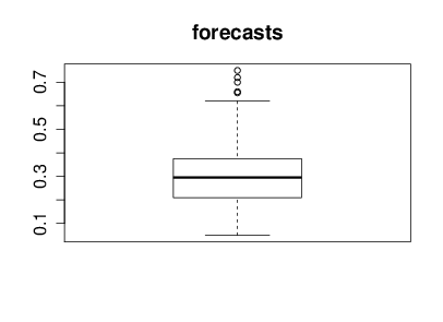
Figure: Summary forecast from those that responded to a scicast question about how consistent the decision making was.

NeurIPS Experiment Results

The results of the experiment were as follows. From 170 papers 4 had to be withdrawn or were rejected without completing the review process, for the remainder, the ‘confusion matrix’ for the two committee’s decisions is in Table .

Table: Table showing the results from the two committees as a confusion matrix. Four papers were rejected or withdrawn without review.

		Committee 1
		Accept	Reject
Committee 2	Accept	22	22
	Reject	21	101

Summarizing the Table

There are a few ways of summarizing the numbers in this table as percent or probabilities. First, the inconsistency, the proportion of decisions that were not the same across the two committees. The decisions were inconsistent for 43 out of 166 papers or 0.259 as a proportion. This number is perhaps a natural way of summarizing the figures if you are submitting your paper and wish to know an estimate of what the probability is that your paper would have different decisions according to the different committees. Secondly, the accept precision: if you are attending the conference and looking at any given paper, then you might want to know the probability that the paper would have been rejected in an independent rerunning of the conference. We can estimate this for Committee 1’s conference as 22/(22 + 22) = 0.5 (50%) and for Committee 2’s conference as 21/(22+21) = 0.49 (49%). Averaging the two estimates gives us 49.5%. Finally, the reject precision: if your paper was rejected from the conference, you might like an estimate of the probability that the same paper would be rejected again if the review process had been independently rerun. That estimate is 101/(22+101) = 0.82 (82%) for Committee 1 and 101/(21+101)=0.83 (83%) for Committee 2, or on average 82.5%. A final quality estimate might be the ratio of consistent accepts to consistent rejects, or the agreed accept rate, 22/123 = 0.18 (18%).

• inconsistency: 43/166 = 0.259
  • proportion of decisions that were not the same
• accept precision \(0.5 \times 22/44\) + \(0.5 \times 21/43\) = 0.495
  • probability any accepted paper would be rejected in a rerunning
• reject precision = \(0.5\times 101/(22+101)\) + \(0.5\times 101/(21 + 101)\) = 0.175
  • probability any rejected paper would be rejected in a rerunning
• agreed accept rate = 22/101 = 0.218
• ratio between agreed accepted papers and agreed rejected papers.

Reaction After Experiment

There seems to have been a lot of discussion of the result, both at the conference and on bulletin boards since. Such discussion is to be encouraged, and for ease of memory, it is worth pointing out that the approximate proportions of papers in each category can be nicely divided in to eighths as follows. Accept-Accept 1 in 8 papers, Accept-Reject 3 in 8 papers, Reject-Reject, 5 in 8 papers. This makes the statistics we’ve computed above: inconsistency 1 in 4 (25%) accept precision 1 in 2 (50%) reject precision 5 in 6 (83%) and agreed accept rate of 1 in 6 (20%). This compares with the accept rate of 1 in 4.

• Public reaction after experiment documented here

• Open Data Science (see Heidelberg Meeting)

• NIPS was run in a very open way. Code and blog posts all available!

• Reaction triggered by this blog post.

Much of the discussion speculates on the number of consistent accepts in the process (using the main conference accept rate as a proxy). It therefore produces numbers that don’t match ours above. This is because the computed accept rate of the individual committees is different from that of the main conference. This could be due to a bias for the duplicated papers, or statistical sampling error. We look at these questions below. First, to get the reader primed for thinking about these numbers we discuss some context for placing these numbers.

A Random Committee @ 25%

The first context we can place around the numbers is what would have happened at the ‘Random Conference’ where we simply accept a quarter of papers at random. In this NIPS the expected numbers of accepts would then have been given as in Table .

Table: Table shows the expected values for the confusion matrix if the committee was making decisions totally at random.

		Committee 1
		Accept	Reject
Committee 2	Accept	10.4 (1 in 16)	31.1 (3 in 16)
	Reject	31.1 (3 in 16)	93.4 (9 in 16)

And for this set up we would expect inconsistency of 3 in 8 (37.5%) accept precision of 1 in 4 (25%) and a reject precision of 3 in 4 (75%) and a agreed accept rate of 1 in 10 (10%). The actual committee made improvements on these numbers, the accept precision was markedly better with 50%: twice as many consistent accept decisions were made than would be expected if the process had been performed at random and only around two thirds as many inconsistent decisions were made as would have been expected if decisions were made at random. However, we should treat all these figures with some skepticism until we’ve performed some estimate of the uncertainty associated with them.

Stats for Random Committee

• For random committee we expect:
  • inconsistency of 3 in 8 (37.5%)
  • accept precision of 1 in 4 (25%)
  • reject precision of 3 in 4 (75%) and a
  • agreed accept rate of 1 in 10 (10%).

Actual committee’s accept precision markedly better with 50% accept precision.

Uncertainty: Accept Rate

To get a handle on the uncertainty around these numbers we’ll start by making use of the binomial distribution. First, let’s explore the fact that for the overall conference the accept rate was around 23%, but for the duplication committees the accept rate was around 25%. If we assume decisions are made according to a binomial distribution, then is the accept rate for the duplicated papers too high?

Note that for all our accept probability statistics we used as a denominator the number of papers that were initially sent for review, rather than the number where a final decision was made by the program committee. These numbers are different because some papers are withdrawn before the program committee makes its decision. Most commonly this occurs after authors have seen their preliminary reviews: for NIPS 2014 we provided preliminary reviews that included paper scores. So for the official accept probability we use the 170 as denominator. The accept probabilities were therefore 43 out of 170 papers (25.3%) for Committee 1 and 44 out of 170 (25.8%) for Committee 2. This compares with the overall conference accept rate for papers outside the duplication process of 349 out of 1508 (23.1%).

If the true underlying probability of an accept were 0.23, independent of the paper, then the probability of generating accepts for any subset of the papers would be given by a binomial distribution. Combining across the two committees for the duplicated papers, we see that 87 papers in total were recommended for accept out of a total of 340 trials. out of 166 trials would be given by a binomial distribution as depicted below.

import numpy as np
from scipy.stats import binom
from IPython.display import HTML

Figure: Number of accepted papers for \(p=0.23\).

From the plot, we can see that whilst the accept rate was slightly higher for duplicated papers it doesn’t seem that we can say that it was statistically significant that it was higher, it falls well within the probability mass of the Binomial.

Note that Area Chairs knew which papers were duplicates, whereas reviewers did not. Whilst we stipulated that duplicate papers should not be any given special treatment, we cannot discount the possibility that Area Chairs may have given slightly preferential treatment to duplicate papers.

Uncertainty: Accept Precision

For the accept precision, if we assume that accept decisions were drawn according to a binomial, then the distribution for consistent accepts is also binomial. Our best estimate of its parameter is 22/166 = 0.13 (13%). If we had a binomial distribution with these parameters, then the distribution of consistent accepts would be as follows.

• How reliable is the consistent accept score?

Figure: Number of consistent accepts given \(p=0.13\).

We see immediately that there is a lot of uncertainty around this number, for the scale of the experiment as we have it. This suggests a more complex analysis is required to extract our estimates with uncertainty.

Bayesian Analysis

Before we start the analysis, it’s important to make some statements about the aims of our modelling here. We will make some simplifying modelling assumptions for the sake of a model that is understandable. We are looking to get a handle on the uncertainty associated with some of the probabilities associated with the NIPS experiment. Some preliminary analyses have already been conducted on blogs. Those analyses don’t have access to information like paper scores etc. For that reason we also leave out such information in this preliminary analysis. We will focus only on the summary results from the experiment: how many papers were consistently accepted, consistently rejected, or had inconsistent decisions. For the moment we disregard the information we have about paper scores.

In our analysis there are three possible outcomes for each paper: consistent accept, inconsistent decision and consistent reject. So, we need to perform the analysis with the multinomial distribution. The multinomial is parameterized by the probabilities of the different outcomes. These are our parameters of interest; we would like to estimate these probabilities alongside their uncertainties. To make a Bayesian analysis we place a prior density over these probabilities, then we update the prior with the observed data, that gives us a posterior density, giving us an uncertainty associated with these probabilities.

Prior Density

Choice of prior for the multinomial is typically straightforward, the Dirichlet density is conjugate and has the additional advantage that its parameters can be set to ensure it is uninformative, i.e. uniform across the domain of the prior. Combination of a multinomial likelihood and a Dirichlet prior is not new, and in this domain if we were to consider the mean the posterior density only, then the approach is known as Laplace smoothing.

For our model we are assuming for our prior that the probabilities are drawn from a Dirichlet as follows, \[ p \sim \text{Dir}(\alpha_1, \alpha_2, \alpha_3), \] with \(\alpha_1=\alpha_2=\alpha_3=1\). The Dirichlet density is conjugate to the multinomial distribution, and we associate three different outcomes with the multinomial. For each of the 166 papers we expect to have a consistent accept (outcome 1), an inconsistent decision (outcome 2) or a consistent reject (outcome 3). If the counts four outcome 1, 2 and 3 are represented by \(k_1\), \(k_2\) and \(k_3\) and the associated probabilities are given by \(p_1\), \(p_2\) and \(p_3\) then our model is, \[\begin{align*} \mathbf{p}|\boldsymbol{\alpha} \sim \text{Dir}(\boldsymbol{\alpha}) \\ \mathbf{k}|\mathbf{p} \sim \text{mult}(\mathbf{p}). \end{align*}\] Due to the conjugacy the posterior is tractable and easily computed as a Dirichlet (see e.g. Gelman et al), where the parameters of the Dirichlet are given by the original vector from the Dirichlet prior plus the counts associated with each outcome. \[ \mathbf{p}|\mathbf{k}, \boldsymbol{\alpha} \sim \text{Dir}(\boldsymbol{\alpha} + \mathbf{k}) \] The mean probability for each outcome is then given by, \[ \bar{p}_i = \frac{\alpha_i+k_i}{\sum_{j=1}^3(\alpha_j + k_j)}. \] and the variance is \[ \mathrm{Var}[p_i] = \frac{(\alpha_i+k_i) (\alpha_0-\alpha_i + n + k_i)}{(\alpha_0+n)^2 (\alpha_0+n+1)}, \] where \(n\) is the number of trials (166 in our case) and \(\alpha_0 = \sum_{i=1}^3\alpha_i\). This allows us to compute the expected value of the probabilities and their variances under the posterior as follows.

def posterior_mean_var(k, alpha):
    """Compute the mean and variance of the Dirichlet posterior."""
    alpha_0 = alpha.sum()
    n = k.sum()
    m = (k + alpha)
    m /= m.sum()
    v = (alpha+k)*(alpha_0 - alpha + n + k)/((alpha_0+n)**2*(alpha_0+n+1))
    return m, v

k = np.asarray([22, 43, 101])
alpha = np.ones((3,))
m, v = posterior_mean_var(k, alpha)
outcome = ['consistent accept', 'inconsistent decision', 'consistent reject']
for i in range(3):
    display(HTML("<h4>Probability of " + outcome[i] +' ' + str(m[i]) +  "+/-" + str(2*np.sqrt(v[i])) + "</h4>"))

So we have a probability of consistent accept as \(0.136 \pm 0.06\), the probability of inconsistent decision as \(0.260 \pm 0.09\) and probability of consistent reject as \(0.60 \pm 0.15\). Recall that if we’d selected papers at random (with accept rate of 1 in 4) then these values would have been 1 in 16 (0.0625), 3 in 8 (0.375) and 9 in 16 (0.5625).

The other values we are interested in are the accept precision, reject precision and the agreed accept rate. Computing the probability density for these statistics is complex: it involves Ratio Distributions. However, we can use Monte Carlo to estimate the expected accept precision, reject precision, and agreed accept rate as well as their variances. We can use these results to give us error bars and histograms of these statistics.

def sample_precisions(k, alpha, num_samps):
    """Helper function to sample from the posterior distibution of accept, 
    reject and inconsistent probabilities and compute other statistics of interest 
    from the samples."""

    k = np.random.dirichlet(k+alpha, size=num_samps)
    # Factors of 2 appear because inconsistent decisions 
    # are being accounted for across both committees.
    ap = 2*k[:, 0]/(2*k[:, 0]+k[:, 1])
    rp = 2*k[:, 2]/(k[:, 1]+2*k[:, 2])
    aa = k[:, 0]/(k[:, 0]+k[:, 2])
    return ap, rp, aa

ap, rp, aa = sample_precisions(k, alpha, 10000)
print(ap.mean(), '+/-', 2*np.sqrt(ap.var()))
print(rp.mean(), '+/-', 2*np.sqrt(rp.var()))
print(aa.mean(), '+/-', 2*np.sqrt(aa.var()))

Giving an accept precision of \(0.51 \pm 0.13\), a reject precision of \(0.82 \pm 0.05\) and an agreed accept rate of \(0.18 \pm 0.07\). Note that the ‘random conference’ values of 1 in 4 for accept precision and 3 in 4 for reject decisions are outside the two standard deviation error bars. If it is preferred medians and percentiles could also be computed from the samples above, but as we will see when we histogram the results the densities look broadly symmetric, so this is unlikely to have much effect.

Histogram of Monte Carlo Results

Just to ensure that the error bars are reflective of the underlying densities we histogram the Monte Carlo results for accept precision, reject precision and agreed accept below. Shown on each histogram is a line representing the result we would get for the ‘random committee.’

Figure: Different statistics for the random committee oucomes versus the observed committee outcomes.

Model Choice and Prior Values

In the analysis above we’ve minimized the modeling choices: we made use of a Bayesian analysis to capture the uncertainty in counts that can be arising from statistical sampling error. To this end we chose an uninformative prior over these probabilities. However, one might argue that the prior should reflect something more about the underlying experimental structure: for example, we know that if the committees made their decisions independently it is unlikely that we’d obtain an inconsistency figure much greater than 37.5% because that would require committees to explicitly collude to make inconsistent decisions: the random conference is the worst case. Due to the accept rate, we also expect a larger number of reject decisions than reject. This also isn’t captured in our prior. Such questions move us into the realms of modeling the process, rather than performing a sensitivity analysis. However, if we wish to model the decision process as a whole, we have a lot more information available, and we should make use of it. The analysis above is intended to exploit our randomized experiment to explore how inconsistent we expect two committees to be. It focusses on that single question; it doesn’t attempt to give answers on what the reasons for that inconsistency are and how it may be reduced. The additional maths was needed only to give a sense of the uncertainty in the figures. That uncertainty arises due to the limited number of papers in the experiment.

Reviewer Calibration

Calibration of reviewers is the process where different interpretations of the reviewing scale are addressed. The tradition of calibration goes at least as far back as John Platt’s Program Chairing, and included a Bayesian model by Ge, Welling and Ghahramani at NeurIPS 2013.

Reviewer Calibration Model

In this note book we deal with reviewer calibration. Our assumption is that the score from the \(j\)th reviwer for the \(i\)th paper is given by \[ y_{i,j} = f_i + b_j + \epsilon_{i, j} \] where \(f_i\) is the ‘objective quality’ of paper \(i\) and \(b_j\) is an offset associated with reviewer \(j\). \(\epsilon_{i,j}\) is a subjective quality estimate which reflects how a specific reviewer’s opinion differs from other reviewers (such differences in opinion may be due to differing expertise or perspective). The underlying ‘objective quality’ of the paper is assumed to be the same for all reviewers and the reviewer offset is assumed to be the same for all papers.

If we have \(n\) papers and \(m\) reviewers, then this implies \(n\) + \(m\) + \(nm\) values need to be estimated. Naturally this is too many, and we can start by assuming that the subjective quality is drawn from a normal density with variance \(\sigma^2\) \[ \epsilon_{i, j} \sim N(0, \sigma^2 \mathbf{I}) \] which reduces us to \(n\) + \(m\) + 1 parameters. Further we can assume that the objective quality is also normally distributed with mean \(\mu\) and variance \(\alpha_f\), \[ f_i \sim N(\mu, \alpha_f) \] this now reduces us to \(m\)+3 parameters. However, we only have approximately \(4m\) observations (4 papers per reviewer) so parameters may still not be that well determined (particularly for those reviewers that have only one review). We, therefore, finally, assume that reviewer offset is normally distributed with zero mean, \[ b_j \sim N(0, \alpha_b), \] leaving us only four parameters: \(\mu\), \(\sigma^2\), \(\alpha_f\) and \(\alpha_b\). Combined together these three assumptions imply that \[ \mathbf{y} \sim N(\mu \mathbf{1}, \mathbf{K}), \] where \(\mathbf{y}\) is a vector of stacked scores \(\mathbf{1}\) is the vector of ones and the elements of the covariance function are given by \[ k(i,j; k,l) = \delta_{i,k} \alpha_f + \delta_{j,l} \alpha_b + \delta_{i, k}\delta_{j,l} \sigma^2, \] where \(i\) and \(j\) are the index of first paper and reviewer and \(k\) and \(l\) are the index of second paper and reviewer. The mean is easily estimated by maximum likelihood and is given as the mean of all scores.

It is convenient to reparametrize slightly into an overall scale \(\alpha_f\), and normalized variance parameters, \[ k(i,j; k,l) = \alpha_f\left(\delta_{i,k} + \delta_{j,l} \frac{\alpha_b}{\alpha_f} + \delta_{i, k}\delta_{j,l} \frac{\sigma^2}{\alpha_f}\right) \] which we rewrite to give two ratios: offset/signal ratio, \(\hat{\alpha}_b\) and noise/signal \(\hat{\sigma}^2\) ratio. \[ k(i,j; k,l) = \alpha_f\left(\delta_{i,k} + \delta_{j,l} \hat{\alpha}_b + \delta_{i, k}\delta_{j,l} \hat{\sigma}^2\right) \] The advantage of this parameterization is it allows us to optimize \(\alpha_f\) directly (with a fixed-point equation) and it will be very well determined. This leaves us with two free parameters, that we can explore on the grid. It is in these parameters that we expect the remaining underdetermindness of the model. We expect \(\alpha_f\) to be well determined because the negative log likelihood is now \[ \frac{|\mathbf{y}|}{2}\log\alpha_f + \frac{1}{2}\log \left|\hat{\mathbf{K}}\right| + \frac{1}{2\alpha_f}\mathbf{y}^\top \hat{\mathbf{K}}^{-1} \mathbf{y}, \] where \(|\mathbf{y}|\) is the length of \(\mathbf{y}\) (i.e. the number of reviews) and \(\hat{\mathbf{K}}=\alpha_f^{-1}\mathbf{K}\) is the scale normalized covariance. This negative log likelihood is easily minimized to recover \[ \alpha_f = \frac{1}{|\mathbf{y}|} \mathbf{y}^\top \hat{\mathbf{K}}^{-1} \mathbf{y}. \] A Bayesian analysis of this parameter is possible with gamma priors, but it would merely show that this parameter is extremely well determined (the degrees of freedom parameter of the associated Student-\(t\) marginal likelihood scales will the number of reviews, which will be around \(|\mathbf{y}| \approx 6,000\) in our case.

So, we propose to proceed as follows. Set the mean from the reviews (\(\mu\)) and then choose a two-dimensional grid of parameters for reviewer offset and diversity. For each parameter choice, optimize to find \(\alpha_f\) and then evaluate the liklihood. Worst case this will require us inverting \(\hat{\mathbf{K}}\), but if the reviewer paper groups are disconnected, it can be done a lot quicker. Next stage is to load in the reviews for analysis.

Fitting the Model

import cmtutils as cu
import os
import pandas as pd
import numpy as np
import GPy
from scipy.sparse.csgraph import connected_components
from scipy.linalg import solve_triangular 

date = '2014-09-06'

Loading in the Data

filename = date + '_reviews.xls'
reviews = cu.CMT_Reviews_read(filename=filename)
papers = list(sorted(set(reviews.reviews.index), key=int))
reviews.reviews = reviews.reviews.loc[papers]

The maximum likelihood solution for \(\mu\) is simply the mean quality of the papers, this is easily computed.

mu = reviews.reviews.Quality.mean()
print("Mean value, mu = ", mu)

Data Preparation

We take the reviews, which are indexed by the paper number, and create a new data frame, that indexes by paper id and email combined. From these reviews we tokenize the PaperID and the Email to extract two matrices that can be used in creation of covariance matrices. We also create a target vector which is the mean centred vector of scores.

r = reviews.reviews.reset_index()
r.rename(columns={'ID':'PaperID'}, inplace=True)
r.index = r.PaperID + '_' + r.Email
X1 = pd.get_dummies(r.PaperID)
X1 = X1[sorted(X1.columns, key=int)]
X2 = pd.get_dummies(r.Email)
X2 = X2[sorted(X2.columns, key=str.lower)]
y = reviews.reviews.Quality - mu

Constructing the Model in GPy

Having reduced the model to two parameters, I was hopeful I could set parameters broadly by hand. My initial expectation was that alpha_b and sigma2 would both be less than 1, but some playing with parameters showed this wasn’t the case. Rather than waste further time, I decided to use our GPy Software (see below) to find a maximum likelihood solution for the parameters.

Model construction firstly involves constructing covariance functions for the model and concatenating X1 and X2 to a new input matrix X.

X = X1.join(X2)
kern1 = GPy.kern.Linear(input_dim=len(X1.columns), active_dims=np.arange(len(X1.columns)))
kern1.name = 'K_f'
kern2 = GPy.kern.Linear(input_dim=len(X2.columns), active_dims=np.arange(len(X1.columns), len(X.columns)))
kern2.name = 'K_b'

Next, the covariance function is used to create a Gaussian process regression model with X as input and y as target. The covariance function is given by \(\mathbf{K}_f + \mathbf{K}_b\).

model = GPy.models.GPRegression(X, y.to_numpy()[:, np.newaxis], kern1+kern2)
model.optimize()

Now we can check the parameters of the result.

print(model)
print(model.log_likelihood())

    Name : GP regression
    Objective : 10071.679092815619
    Number of Parameters : 3
    Number of Optimization Parameters : 3
    Updates : True
    Parameters:
      GP_regression.           |               value  |  constraints  |  priors
      sum.K_f.variances        |  1.2782303448777643  |      +ve      |        
      sum.K_b.variances        |  0.2400098787580176  |      +ve      |        
      Gaussian_noise.variance  |  1.2683656892796749  |      +ve      |        
    -10071.679092815619

Construct the Model Without GPy

The answer from the GPy solution is introduced here, alongside the code where the covariance matrices are explicitly created (above they are created using GPy’s high level code for kernel matrices, which may be less clear on the details).

# set parameter values to ML solutions given by GPy.
alpha_f = model.sum.K_f.variances
alpha_b = model.sum.K_b.variances/alpha_f
sigma2 = model.Gaussian_noise.variance/alpha_f

Now we create the covariance functions based on the tokenized paper IDs and emails.

K_f = np.dot(X1, X1.T)
K_b = alpha_b*np.dot(X2, X2.T)
K = K_f + K_b + sigma2*np.eye(X2.shape[0])
Kinv, L, Li, logdet = GPy.util.linalg.pdinv(K) # since we have GPy loaded in use their positive definite inverse.
y = reviews.reviews.Quality - mu
alpha = np.dot(Kinv, y)
yTKinvy = np.dot(y, alpha)
alpha_f = yTKinvy/len(y)

Since we have removed the data mean, the log likelihood we are interested in is the likelihood of a multivariate Gaussian with covariance \(\mathbf{K}\) and mean zero. This is computed below.

ll = 0.5*len(y)*np.log(2*np.pi*alpha_f) + 0.5*logdet + 0.5*yTKinvy/alpha_f 
print("negative log likelihood: ", ll)

Review Quality Prediction

Now we wish to predict the bias corrected scores for the papers. That involves considering a variable \(s_{i,j} = f_i + e_{i,j}\) which is the score with the bias removed. That variable has a covariance matrix, \(\mathbf{K}_s=\mathbf{K}_f + \sigma^2 \mathbf{I}\) and a cross covariance between \(\mathbf{y}\) and \(\mathbf{s}\) is also given by \(\mathbf{K}_s\). This means we can compute the posterior distribution of the scores as follows:

# Compute mean and covariance of quality scores
K_s = K_f + np.eye(K_f.shape[0])*sigma2
s = pd.Series(np.dot(K_s, alpha) + mu, index=X1.index)
covs = alpha_f*(K_s - np.dot(K_s, np.dot(Kinv, K_s)))

Monte Carlo Simulations for Probability of Acceptance

We can now sample from this posterior distribution of bias-adjusted scores jointly, to get a set of scores for all papers. For this set of scores, we can perform a ranking and accept the top 400 papers. This gives us a sampled conference. If we do that 1,000 times then we can see how many times each paper was accepted to get a probability of acceptance.

number_accepts = 420 # 440 because of the 10% replication

# place this in a separate box, because sampling can take a while.
samples = 1000
score = np.random.multivariate_normal(mean=s, cov=covs, size=samples).T
# Use X1 which maps papers to paper/reviewer pairings to get the average score for each paper.
paper_score = pd.DataFrame(np.dot(np.diag(1./X1.sum(0)), np.dot(X1.T, score)), index=X1.columns)

Now we can compute the probability of acceptance for each of the sampled rankings.

prob_accept = ((paper_score>paper_score.quantile(1-(float(number_accepts)/paper_score.shape[0]))).sum(1)/1000)
prob_accept.name = 'AcceptProbability'

Now we have the probability of accepts, we can decide on the boundaries of the grey area. These are set in lower and upper. The grey area is those papers that will be debated most heavily during the teleconferences between program chairs and area chairs.

lower=0.1
upper=0.9
grey_area = ((prob_accept>lower) & (prob_accept<upper))
print('Number of papers in grey area:', grey_area.sum())

import matplotlib.pyplot as plt
import cmtutils.plot as plot

fig, ax = plt.subplots(figsize=plot.big_wide_figsize)
print('Expected Papers Accepted:', prob_accept.sum())
_ = prob_accept.hist(bins=40, ax=ax)
ma.write_figure(directory="./neurips", filename="probability-of-accept.svg")

Figure: Histogram of the probability of accept as estimated by the Monte Carlo simulation across all papers submitted to NeurIPS 2014.

Some Sanity Checking Plots

Here is the histogram of the reviewer scores after calibration.

fig, ax = plt.subplots(figsize=plot.big_wide_figsize)
s.hist(bins=100, ax=ax)
_ = ax.set_title('Calibrated Reviewer Scores')
ma.write_figure(directory="./neurips", filename="calibrated-reviewer-scores.svg")

Figure: Histogram of updated reviewer scores after the calibration process is applied.

Adjustments to Reviewer Scores

We can also compute the posterior distribution for the adjustments to the reviewer scores.

# Compute mean and covariance of review biases
b = pd.Series(np.dot(K_b, alpha), index=X2.index)
covb = alpha_f*(K_b - np.dot(K_b, np.dot(Kinv, K_b)))

reviewer_bias = pd.Series(np.dot(np.diag(1./X2.sum(0)), np.dot(X2.T, b)), index=X2.columns, name='ReviewerBiasMean')
reviewer_bias_std = pd.Series(np.dot(np.diag(1./X2.sum(0)), np.dot(X2.T, np.sqrt(np.diag(covb)))), index=X2.columns, name='ReviewerBiasStd')

Here is a histogram of the mean adjustment for the reviewers.

fig, ax = plt.subplots(figsize=plot.big_wide_figsize)
reviewer_bias.hist(bins=100, ax=ax)
_ = ax.set_title('Reviewer Calibration Adjustments Histogram')
ma.write_figure(directory="./neurips", filename="reviewer-calibration-adjustments.svg")

Figure: Histogram of individual offsets associated with the reviewers as estimated by the model.

Export a version of the bias scores for use in CMT.

bias_export = pd.DataFrame(data={'Quality Score - Does the paper deserves to be published?':reviewer_bias, 
                   'Impact Score - Independently of the Quality Score above, this is your opportunity to identify papers that are very different, original, or otherwise potentially impactful for the NIPS community.':pd.Series(np.zeros(len(reviewer_bias)), index=reviewer_bias.index),
                    'Confidence':pd.Series(np.zeros(len(reviewer_bias)), index=reviewer_bias.index)})
cols = bias_export.columns.tolist()
cols = [cols[2], cols[1], cols[0]]
bias_export = bias_export[cols]
#bias_export.to_csv(os.path.join(cu.cmt_data_directory, 'reviewer_bias.csv'), sep='\t', header=True, index_label='Reviewer Email')

Sanity Check

As a sanity check Corinna suggested it makes sense to plot the average raw score for the papers vs the probability of accept, just to ensure nothing weird is going on. To clarify the plot, I’ve actually plotted raw score vs log odds of accept.

raw_score = pd.Series(np.dot(np.diag(1./X1.sum(0)), np.dot(X1.T, r.Quality)), index=X1.columns)
prob_accept[prob_accept==0] = 1/(10*samples)
prob_accept[prob_accept==1] = 1-1/(10*samples)

fig, ax = plt.subplots(figsize=plot.big_wide_figsize)
ax.plot(raw_score, np.log(prob_accept)- np.log(1-prob_accept), 'rx')
ax.set_title('Raw Score vs Log odds of accept')
ax.set_xlabel('raw score')
_ = ax.set_ylabel('log odds of accept')
ma.write_figure(directory="./neurips", filename="raw-score-vs-log-odds.svg")

Figure: Scatter plot of the raw paper score against the log probability of paper acceptance, as estimated by Monte Carlo simulation.

Calibraton Quality Sanity Checks

s.name = 'CalibratedQuality'
r = r.join(s)

We can also look at a scatter plot of the review quality vs the calibrated quality.

fig, ax = plt.subplots(figsize=plot.big_wide_figsize)
ax.plot(r.Quality, r.CalibratedQuality, 'r.', markersize=10)
ax.set_xlim([0, 11])
ax.set_xlabel('original review score')
_ = ax.set_ylabel('calibrated review score')
ma.write_figure(directory="./neurips", filename="calibrated-review-score-vs-original-score.svg")

Figure: Scatter plot of the calibrated review scores against the original review scores.

Correlation of Duplicate Papers

For NeurIPS 2014 we experimented with duplicate papers: we pushed papers through the system twice, exposing them to different subsets of the reviewers. The first thing we’ll look at is the duplicate papers. Firstly, we identify them by matching on title.

filename = date + '_paper_list.xls'
papers = cu.CMT_Papers_read(filename=filename)
duplicate_list = []
for ID, title in papers.papers.Title.iteritems():
    if int(ID)>1779 and int(ID) != 1949:
        pair = list(papers.papers[papers.papers['Title'].str.contains(papers.papers.Title[ID].strip())].index)
        pair.sort(key=int)
        duplicate_list.append(pair)

Next, we compute the correlation coefficients for the duplicated papers for the average impact and quality scores.

quality = []
calibrated_quality = []
accept = []
impact = []
confidence = []
for duplicate_pair in duplicate_list:
    quality.append([np.mean(r[r.PaperID==duplicate_pair[0]].Quality), np.mean(r[r.PaperID==duplicate_pair[1]].Quality)])
    calibrated_quality.append([np.mean(r[r.PaperID==duplicate_pair[0]].CalibratedQuality), np.mean(r[r.PaperID==duplicate_pair[1]].CalibratedQuality)])
    impact.append([np.mean(r[r.PaperID==duplicate_pair[0]].Impact), np.mean(r[r.PaperID==duplicate_pair[1]].Impact)])
    confidence.append([np.mean(r[r.PaperID==duplicate_pair[0]].Conf), np.mean(r[r.PaperID==duplicate_pair[1]].Conf)])
quality = np.array(quality)
calibrated_quality = np.array(calibrated_quality)
impact = np.array(impact)
confidence = np.array(confidence)
quality_cor = np.corrcoef(quality.T)[0, 1]
calibrated_quality_cor = np.corrcoef(calibrated_quality.T)[0, 1]
impact_cor = np.corrcoef(impact.T)[0, 1]
confidence_cor = np.corrcoef(confidence.T)[0, 1]
print("Quality correlation: ", quality_cor)
print("Calibrated Quality correlation: ", calibrated_quality_cor)
print("Impact correlation: ", impact_cor)
print("Confidence correlation: ", confidence_cor)

    Quality correlation:  0.54403674862622
    Calibrated Quality correlation:  0.5455958618174274
    Impact correlation:  0.26945269236041036
    Confidence correlation:  0.3854251559444674

Correlation Plots

To visualize the quality score correlation, we plot the group 1 papers against the group 2 papers. Here we add a small amount of jitter to ensure points to help visualize points that would otherwise fall on the same position.

Figure: Correlation between reviewer scores across the duplicated committees (scores have jitter added to prevent too many points sitting on top of each other).

Similarly for the calibrated quality of the papers.

Figure: Correlation between calibrated reviewer scores across the two independent committees.

# Apply Laplace smoothing to accept probabilities before incorporating them.
revs = r.join((prob_accept+0.0002)/1.001, on='PaperID').join(reviewer_bias, on='Email').join(papers.papers['Number Of Discussions'], on='PaperID').join(reviewer_bias_std, on='Email').sort_values(by=['AcceptProbability','PaperID', 'CalibratedQuality'], ascending=False)
revs.set_index(['PaperID'], inplace=True)
def len_comments(x):
    return len(x.Comments)
revs['comment_length']=revs.apply(len_comments, axis=1)
# Save the computed information to disk
#revs.to_csv(os.path.join(cu.cmt_data_directory, date + '_processed_reviews.csv'), encoding='utf-8')

Conference Simulation

Given the realization that roughly 50% of the score seems to be ‘subjective’ and 50% of the score seems to be ‘objective,’ then we can simulate the conference and see what it does for the consistency of accepts for different probability of accept.

import numpy as np

samples = 100000
subjectivity_portion = 0.5

accept_rates = [0.05, 0.1, 0.15, 0.2, 0.25, 0.3, 0.35, 0.4, 0.45, 0.5, 0.55, 0.6, 0.65, 0.7, 0.75, 0.8, 0.85, 0.9, 0.95, 1.0]
consistent_accepts = []
for accept_rate in accept_rates:
    score_1 = []
    score_2 = []
    for i in range(samples):
        objective = (1-subjectivity_portion)*np.random.randn()
        score_1.append(objective + subjectivity_portion*np.random.randn())
        score_2.append(objective + subjectivity_portion*np.random.randn())

    score_1 = np.asarray(score_1)
    score_2 = np.asarray(score_2)

    accept_1 = score_1.argsort()[:int(samples*accept_rate)]
    accept_2 = score_2.argsort()[:int(samples*accept_rate)]

    consistent_accept = len(set(accept_1).intersection(set(accept_2)))
    consistent_accepts.append(consistent_accept/(samples*accept_rate))
    print('Percentage consistently accepted: {prop}'.format(prop=consistent_accept/(samples*accept_rate)))

consistent_accepts = np.array(consistent_accepts)
accept_rate = np.array(accept_rate)

Figure: Plot of the accept rate vs the consistency of the conference for 50% subjectivity.

Figure: Plot of the accept rate vs gain in consistency over a random conference for 50% subjectivity.

Where do Rejected Papers Go?

import os
import yaml

with open(os.path.join(nipsy.review_store, nipsy.outlet_name_mapping), 'r') as f:
    mapping = yaml.load(f, Loader=yaml.FullLoader)


date = "2021-06-11"

citations = nipsy.load_citation_counts(date=date)
decisions = nipsy.load_decisions()
nipsy.augment_decisions(decisions)
joindf = nipsy.join_decisions_citations(decisions, citations)

joindf['short_venue'] = joindf.venue.replace(mapping)

fig = go.Figure(data=data,
                layout = go.Layout(width=600,
                height=450))
fig.update_layout(template="plotly", font=dict(
        family="sans serif",
        size=14,
        color="Black"
    ))
fig.show()
fig.write_html(os.path.join(".", "./neurips", "where-do-neurips-papers-go.html"))
fig.write_image(os.path.join(".", "./neurips", "where-do-neurips-papers-go.svg"))

Figure: Sankey diagram showing the flow of NeurIPS papers through the system from submission to eventual publication.

Effect of Late Reviews

This notebook analyzes the reduction in reviewer confidence between reviewers that submit their reviews early and those that arrive late. The reviews are first loaded in from files Corinna and Neil saved and stored in a pickle. The function for doing that is nips.load_review_history.

import cmtutils as cu
import cmtutils.nipsy as nipsy 
import cmtutils.plot as plot

import os
import pandas as pd
import numpy as np

reviews = nipsy.load_review_history()

Review Submission Times

All reviews are now in pandas data frame called reviews, they are ready for processing. First of all, let's take a look at when the reviews were submitted. The function nipsy.reviews_before gives a snapshot of the reviews as they stood at a particular date. So we simply create a data series across the data range of reviews (nipsy.review_data_range) that shows the counts.

review_count = pd.Series(index=nipsy.review_date_range)
for date in nipsy.review_date_range:
    review_count.loc[date] = nipsy.reviews_before(reviews, date).Quality.shape[0]

Figure: Cumulative count of number of received reviews over time.

We worked hard to try and ensure that all papers had three reviews before the start of the rebuttal. This next plot shows the numbers of papers that had less than three reviews across the review period. First let’s look at the overall statistics of what the count of reviewers per paper were. Below we plot mean, maximum, median, and minimum over time.

lastseen = reviews.drop_duplicates(subset='ID').set_index('ID')
lastseen = lastseen['LastSeen']

review_count = pd.DataFrame(index=reviews.ID.unique(), columns=nipsy.review_date_range)
for date in nipsy.review_date_range:
    counts = nipsy.reviews_status(reviews, date, column='Quality').count(level='ID')
    review_count[date] = counts.fillna(0)
review_count.fillna(0, inplace=True)    
review_count = review_count.T
for col in review_count.columns:
    if pd.notnull(lastseen[col]):
        review_count[col][review_count.index>lastseen[col]] = np.NaN
        
review_count = review_count.T

Figure: Plot representing number of reviewers per paper over time showing maximum number of reviewers per paper, minimum, median, and mean.

But perhaps the more important measure is how many papers had less than 3 reviewers over time. In this plot you can see that by the time rebuttal starts almost all papers have three reviewers.

count = pd.Series(index=nipsy.review_date_range)
for date in nipsy.review_date_range:
    count[date] = (review_count[date]<3).sum()

Figure: Number of papers with less than three reviewers as a function of time.

Review Confidence

Now we will check the confidence of reviews as the come in over time. We’ve written a small helper function that looks in a four-day window around each time point and summarises the associated score (in the first case, confidence, Conf) with its across the four day window and 95% confidence intervals computed from the standard error of the mean estimate.

Figure: Average confidence of reviews as computed across a four-day moving window, plot includes sandard error the mean estimate.

It looks like there might be a reduction in confidence as we pass the review deadline on 21st July, but is the difference in confidence for the reviews that came in later significant?

We now simplify the question by looking at the average confidence for reviews that arrived before 21st July (the reviewing deadline) and reviews that arrived after the 21st July (i.e. those that were chased or were allocated late) but before the rebuttal period started (4th August). Below we select these two groups and estimate the estimate of the mean confidence with (again with error bars).

Figure: Average confindence for reviews that arrived before 21st July (the reviewing deadline) and reviews that arrived after. Histogram shows mean values and confidence intervals. A \(t\)-test shows the difference to be significant with a \(p\)-value of 0.048%, although the magnitude of the difference is small (about 0.1).

So, it looks like there is a small but significant difference between the average confidence of the submitted reviews before and after the deadline, the statistical significance is confirmed with a \(t\)-test with a \(p\)-value at 0.048%. The magnitude of the difference is small (about 0.1) but may indicate a tendency for later reviewers to be a little more rushed.

Quality Score

This begs the question, is there an effect on the other scores of their reviews which cover ‘quality’ and ‘impact.’ Quality of papers is scored on a 10-point scale with a recommendation of 6 being accept and We can form a similar plots for quality as shown in Figures and .

Figure: Plot of average review quality score as a function of time using a four day moving window. Standard error is also shown in the plot.

Figure: Bar plot of average quality scores for on-time reviews and late reviews, standard errors shown. Under a \(t\)-test the difference in values is statistically significant with a \(p\)-value of 0.007%.

There is another statistically significant difference between perceived quality scores after the reviewing deadline than before. On average reviewers tend to be more generous in their quality perceptions when the review is late. The \(p\)-value is computed as 0.007%. We can also check if there is a similar on the impact score. The impact score was introduced by Ghahramani and Welling to get reviewers not just to think about the technical side of the paper, but whether it is driving the field forward. The score is binary, with 1 being for a paper that is unlikely to have high impact and 2 being for a paper that is likely to have a high impact.

Figure: Average impact score for papers over time, again using a moving average with a window of four days and with standard error of the mean computation shown.

Figure: Bar plot showing the average impact score of reviews submitted before the deadline and after the deadline. The difference in means did not prove to be statistically significant under a \(t\)-test (\(p\)-value 5.9%).

We find the difference is not quite statistically significant for the impact score (\(p\)-value of 5.9%), but if anything, there is a trend to have slightly higher impacts for later reviews (see Figures and ).

Review Length

A final potential indicator of review quality is the length of the reviews, we can check if there is a difference between the combined length of the review summary and the main body comments for late and early reviews (see Figures and ).

Figure: Average length of reviews submitted plotted as a function of time with standard error of the mean computation included.

Figure: Bar plot of the average length of reviews submitted before and after the deadline with standard errors included. The difference of around 100 words is statistically significant under a \(t\)-test (\(p\)-value 0.55%).

Once again we find a small but statistically significant difference, here, as we might expect late reviews are shorter than those submitted on time, by about 100 words in a 2,400 word review.

review_quality = pd.DataFrame(index=reviews.ID.unique(), columns=nipsy.review_date_range)
for date in nipsy.review_date_range:
    qual = nipsy.reviews_status(reviews, date, column='Quality')
    review_quality[date] = qual.sum(level='ID')/qual.count(level='ID') # There's a bug where mean doesn't work in Pandas 1.2.4??

original_pairs = pd.read_csv(os.path.join(nipsy.review_store, 'Duplicate_PaperID_Pairs.csv'), index_col='original')
duplicate_pairs = pd.read_csv(os.path.join(nipsy.review_store, 'Duplicate_PaperID_Pairs.csv'), index_col='duplicate')

Perform an ‘inner join’ on duplicate papers and their originals with their reviews, and set the index of the duplicated papers to match the original. This gives us data frames with matching indices containing scores over time of the duplicate and original papers.

duplicate_reviews = duplicate_pairs.join(review_quality, how="inner").set_index('original')
original_reviews = original_pairs.join(review_quality, how="inner")
del original_reviews["duplicate"]

corr_series = duplicate_reviews.corrwith(original_reviews)
corr_series.index = pd.to_datetime(corr_series.index)

bootstrap_corr_df = pd.DataFrame(index=corr_series.index)
for i in range(1000):
    ind = bootstrap_index(original_reviews)
    b_corr_series = duplicate_reviews.loc[ind].corrwith(original_reviews.loc[ind])
    b_corr_series.index = pd.to_datetime(b_corr_series.index)
    bootstrap_corr_df[i] = b_corr_series

import datetime as dt

Figure: Average correlation of duplicate papers over time. To give an estimate of the uncertainty the correlation is computed with bootstrap samples. Here to allow comparison between the trend lines similar, the bootstrap samples are set so they converge on the same point on the right of the graph.

Figure: Average correlation of duplicate papers over time.

We need to do a bit more analysis on the estimation of the correlation for the earlier submissions, but from what we see above, it looks like the correlation is being damaged by late reviews, and we never quite recover the consistency of reviews we had at the submission deadline even after the discussion phase is over.

Late Reviewers Summary

In summary we find that late reviews are on average less confident and shorter, but rate papers as higher quality and perhaps as higher impact. Each of the effects is small (around 5%) but overall a picture emerges of a different category of review from those that delay their assessment.

Impact of Papers Seven Years On

Now we look at the actual impact of the papers published using the Semantic Scholar data base for tracking citations.

import cmtutils as cu
import cmtutils.nipsy as nipsy
import cmtutils.plot as plot

import pandas as pd
import numpy as np

papers = cu.Papers()

https://proceedings.neurips.cc/paper/2014

UPDATE_IMPACTS = False # Set to True to download impacts from Semantic Scholar

The impact of the different papers is downloaded from Semantic scholar using their REST API. This can take some time, and they also throttle the calls. At the moment the code below deosn’t handle the throttling correctly. However, you it will load the cached version of of citations scores from the given date.

if UPDATE_IMPACTS:
    from datetime import datetime
    date=datetime.today().strftime('%Y-%m-%d')
else:
    date = "2021-06-11"

# Rerun to download impacts from Semantic Scholar
if UPDATE_IMPACTS:
    semantic_ids = nipsy.load_semantic_ids()
    citations_dict = citations.to_dict(orient='index')
    # Need to be a bit cleverer here. Semantic scholar will throttle this call.
    sscholar = nipsy.download_citation_counts(citations_dict=citations_dict, semantic_ids=semantic_ids)
    citations = pd.DataFrame.from_dict(citations_dict, orient="index") 
    citations.to_pickle(date + '-semantic-scholar-info.pickle')
else: 
    citations = nipsy.load_citation_counts(date=date)

The final decision sheet provides information about what happened to all of the papers.

decisions = nipsy.load_decisions()
nipsy.augment_decisions(decisions)

This is joined with the citation information to provide our main ability to understand the impact of these papers.

joindf = nipsy.join_decisions_citations(decisions, citations)

Correlation of Quality Scores and Citation

Our first study will be to check the correlation between quality scores of papers and how many times that the papers have been cited in practice. In the plot below, rejected papers are given as crosses, accepted papers are given as dots. We include all papers, whether published in a venue or just available through ArXiv or other preprint servers. We show the published/non-published quality scores and \(\log_{10}(1+\text{citations})\) for all papers in the plot below. In the plot we are showing each point corrupted by some Laplacian noise and also removing axes. The idea is to give a sense of the distribution rather than reveal the score of a particular paper.

Figure: Scatter plot of \(\log_{10}(1+\text{citations})\) against the average calibrated quality score for all papers. To prevent reidentification of individual papers quality scores and citation count, each point is corrupted by differentially private noise in the plot (correlation is computed before adding differentially private noise).

The correlation seems strong, but of course, we are looking at papers which were accepted and rejected by the conference. This is dangerous, as it is quite likely that presentation at the conference may provide some form of lift to the papers’ numbers of citations. So, the right thing to do is to look at the groups separately.

Looking at the accepted papers only shows a very different picture. There is very little correlation between accepted papers’ quality scores and the number of citations they receive.

Figure: Scatter plot of \(\log_{10}(1+\text{citations})\) against the average calibrated quality score for accepted papers. To prevent reidentification of individual papers quality scores and citation count, each point is corrupted by differentially private noise in the plot (correlation is computed before adding differentially private noise).

Conversely, looking at rejected papers only, we do see a slight trend, with higher scoring papers achieving more citations on average. This, combined with the lower average number of citations in the rejected paper group, alongside their lower average scores, explains the correlation we originally observed.

Figure: Scatter plot of \(\log_{10}(1+\text{citations})\) against the average calibrated quality score for rejected papers. To prevent reidentification of individual papers quality scores and citation count, each point is corrupted by differentially private noise in the plot (correlation is computed before adding differentially private noise).

Welling and Ghahramani introduced an “impact” score in NeurIPS 2013, we might expect the impact score to show correlation. And indeed, despite the lower range of the score (a reviewer can score either 1 or 2) we do see some correlation, although it is relatively weak.

Figure: Scatter plot of \(\log_{10}(1+\text{citations})\) against the average impact score for accepted papers. To prevent reidentification of individual papers quality scores and citation count, each point is corrupted by differentially private noise in the plot (correlation is computed before adding differentially private noise).

Finally, we also looked at correlation between the confidence score and the impact. Here correlation is somewhat stronger. Why should confidence be an indicator of higher citations? A plausible explanation is that there is confounder driving both variables. For example, it might be that papers which are easier to understand (due to elegance of the idea, or quality of exposition) inspire greater reviewer confidence and increase the number of citations.

Figure: Scatter plot of \(\log_{10}(1+\text{citations})\) against the average confidence score for accepted papers. To prevent reidentification of individual papers quality scores and citation count, each point is corrupted by differentially private noise in the plot (correlation is computed before adding differentially private noise).

for column in ["average_quality", "average_impact", "average_confidence"]:
    cor = []
    for i in range(1000):
        ind = bootstrap_index(joindf.loc[joindf.accept])
        cor.append(joindf.loc[ind][column].corr(np.log(1+joindf.loc[ind]['numCitedBy'])))
    cora = np.array(cor)
    rho = cora.mean()
    twosd = 2*np.sqrt(cora.var())
    print("{column}".format(column=column.replace("_", " ")))
    print("Mean correlation is {rho} +/- {twosd}".format(rho=rho, twosd=twosd))

Conclusion

Under the simple model we have outlined, we can be confident that there is inconsistency between two independent committees, but the level of inconsistency is much less than we would find for a random committee. If we accept that the bias introduced by the Area Chairs knowing when they were dealing with duplicates was minimal, then if we were to revisit the NIPS 2014 conference with an independent committee then we would expect between 38% and 64% of the presented papers to be the same. If the conference was run at random, then we would only expect 25% of the papers to be the same.

It’s apparent from comments and speculation about what these results mean, that some people might be surprised by the size of this figure. However, it only requires a little thought to see that this figure is likely to be large for any highly selective conference if there is even a small amount of inconsistency in the decision-making process. This is because once the conference has chosen to be ‘highly selective’ then because, by definition, only a small percentage of papers are to be accepted. Now if we think of a type I error as accepting a paper which should be rejected, such errors are easier to make because, again by definition, many more papers should be rejected. Type II errors (rejecting a paper that should be accepted) are less likely because (by setting the accept rate low) there are fewer papers that should be accepted in the first place. When there is a difference of opinion between reviewers, it does seem that many of the aruguments can be distilled down to (a subjective opinion) about whether controlling for type I or type II errors is more important. Further, normally when discussing type I and type II errors we believe that the underlying system of study is genuinely binary: e.g., diseased or not diseased. However, for conferences the accept/reject boundary is not a clear separation point, there is a continuum (or spectrum) of paper quality (as there also is for some diseases). And the decision boundary often falls in a region of very high density.

I would prefer a world were a conference is no longer viewed as a proxy for research quality. The true test of quality is time. In the current world, papers from conferences such as NeurIPS are being used to judge whether a researcher is worthy of a position at a leading company, or whether a researcher gets tenure. This is problematic and damaging for the community. Reviewing is an inconsistent process, but that is not a bad thing. It is far worse to have a reviewing system that is consistently wrong than one which is inconsistently wrong.

My own view of a NeurIPS paper is inspired by the Millenium Galleries in Sheffield. There, among the exhibitions they sometimes have work done by apprentices in their ‘qualification.’ Sheffield is known for knives, and the work of the apprentices in making knives is sometimes very intricate indeed. But it does lead to some very impractical knives. NeurIPS seems to be good at judging technical skill, but not impact. And I suspect the same is true of many other meetings. So, a publication a NeurIPS does seem to indicate that the author has some of the skills required, but it does not necessarily imply that the paper will be impactful.

Thanks!

For more information on these subjects and more you might want to check the following resources.

• twitter: @lawrennd
• podcast: The Talking Machines
• newspaper: Guardian Profile Page
• blog: http://inverseprobability.com

References