\[\newcommand{\tk}[1]{} %\newcommand{\tk}[1]{\textbf{TK}: #1} \newcommand{\Amatrix}{\mathbf{A}} \newcommand{\KL}[2]{\text{KL}\left( #1\,\|\,#2 \right)} \newcommand{\Kaast}{\kernelMatrix_{\mathbf{ \ast}\mathbf{ \ast}}} \newcommand{\Kastu}{\kernelMatrix_{\mathbf{ \ast} \inducingVector}} \newcommand{\Kff}{\kernelMatrix_{\mappingFunctionVector \mappingFunctionVector}} \newcommand{\Kfu}{\kernelMatrix_{\mappingFunctionVector \inducingVector}} \newcommand{\Kuast}{\kernelMatrix_{\inducingVector \bf\ast}} \newcommand{\Kuf}{\kernelMatrix_{\inducingVector \mappingFunctionVector}} \newcommand{\Kuu}{\kernelMatrix_{\inducingVector \inducingVector}} \newcommand{\Kuui}{\Kuu^{-1}} \newcommand{\Qaast}{\mathbf{Q}_{\bf \ast \ast}} \newcommand{\Qastf}{\mathbf{Q}_{\ast \mappingFunction}} \newcommand{\Qfast}{\mathbf{Q}_{\mappingFunctionVector \bf \ast}} \newcommand{\Qff}{\mathbf{Q}_{\mappingFunctionVector \mappingFunctionVector}} \newcommand{\aMatrix}{\mathbf{A}} \newcommand{\aScalar}{a} \newcommand{\aVector}{\mathbf{a}} \newcommand{\acceleration}{a} \newcommand{\bMatrix}{\mathbf{B}} \newcommand{\bScalar}{b} \newcommand{\bVector}{\mathbf{b}} \newcommand{\basisFunc}{\phi} \newcommand{\basisFuncVector}{\boldsymbol{ \basisFunc}} \newcommand{\basisFunction}{\phi} \newcommand{\basisLocation}{\mu} \newcommand{\basisMatrix}{\boldsymbol{ \Phi}} \newcommand{\basisScalar}{\basisFunction} \newcommand{\basisVector}{\boldsymbol{ \basisFunction}} \newcommand{\activationFunction}{\phi} \newcommand{\activationMatrix}{\boldsymbol{ \Phi}} \newcommand{\activationScalar}{\basisFunction} \newcommand{\activationVector}{\boldsymbol{ \basisFunction}} \newcommand{\bigO}{\mathcal{O}} \newcommand{\binomProb}{\pi} \newcommand{\cMatrix}{\mathbf{C}} \newcommand{\cbasisMatrix}{\hat{\boldsymbol{ \Phi}}} \newcommand{\cdataMatrix}{\hat{\dataMatrix}} \newcommand{\cdataScalar}{\hat{\dataScalar}} \newcommand{\cdataVector}{\hat{\dataVector}} \newcommand{\centeredKernelMatrix}{\mathbf{ \MakeUppercase{\centeredKernelScalar}}} \newcommand{\centeredKernelScalar}{b} \newcommand{\centeredKernelVector}{\centeredKernelScalar} \newcommand{\centeringMatrix}{\mathbf{H}} \newcommand{\chiSquaredDist}[2]{\chi_{#1}^{2}\left(#2\right)} \newcommand{\chiSquaredSamp}[1]{\chi_{#1}^{2}} \newcommand{\conditionalCovariance}{\boldsymbol{ \Sigma}} \newcommand{\coregionalizationMatrix}{\mathbf{B}} \newcommand{\coregionalizationScalar}{b} \newcommand{\coregionalizationVector}{\mathbf{ \coregionalizationScalar}} \newcommand{\covDist}[2]{\text{cov}_{#2}\left(#1\right)} \newcommand{\covSamp}[1]{\text{cov}\left(#1\right)} \newcommand{\covarianceScalar}{c} \newcommand{\covarianceVector}{\mathbf{ \covarianceScalar}} \newcommand{\covarianceMatrix}{\mathbf{C}} \newcommand{\covarianceMatrixTwo}{\boldsymbol{ \Sigma}} \newcommand{\croupierScalar}{s} \newcommand{\croupierVector}{\mathbf{ \croupierScalar}} \newcommand{\croupierMatrix}{\mathbf{ \MakeUppercase{\croupierScalar}}} \newcommand{\dataDim}{p} \newcommand{\dataIndex}{i} \newcommand{\dataIndexTwo}{j} \newcommand{\dataMatrix}{\mathbf{Y}} \newcommand{\dataScalar}{y} \newcommand{\dataSet}{\mathcal{D}} \newcommand{\dataStd}{\sigma} \newcommand{\dataVector}{\mathbf{ \dataScalar}} \newcommand{\decayRate}{d} \newcommand{\degreeMatrix}{\mathbf{ \MakeUppercase{\degreeScalar}}} \newcommand{\degreeScalar}{d} \newcommand{\degreeVector}{\mathbf{ \degreeScalar}} % Already defined by latex %\newcommand{\det}[1]{\left|#1\right|} \newcommand{\diag}[1]{\text{diag}\left(#1\right)} \newcommand{\diagonalMatrix}{\mathbf{D}} \newcommand{\diff}[2]{\frac{\text{d}#1}{\text{d}#2}} \newcommand{\diffTwo}[2]{\frac{\text{d}^2#1}{\text{d}#2^2}} \newcommand{\displacement}{x} \newcommand{\displacementVector}{\textbf{\displacement}} \newcommand{\distanceMatrix}{\mathbf{ \MakeUppercase{\distanceScalar}}} \newcommand{\distanceScalar}{d} \newcommand{\distanceVector}{\mathbf{ \distanceScalar}} \newcommand{\eigenvaltwo}{\ell} \newcommand{\eigenvaltwoMatrix}{\mathbf{L}} \newcommand{\eigenvaltwoVector}{\mathbf{l}} \newcommand{\eigenvalue}{\lambda} \newcommand{\eigenvalueMatrix}{\boldsymbol{ \Lambda}} \newcommand{\eigenvalueVector}{\boldsymbol{ \lambda}} \newcommand{\eigenvector}{\mathbf{ \eigenvectorScalar}} \newcommand{\eigenvectorMatrix}{\mathbf{U}} \newcommand{\eigenvectorScalar}{u} \newcommand{\eigenvectwo}{\mathbf{v}} \newcommand{\eigenvectwoMatrix}{\mathbf{V}} \newcommand{\eigenvectwoScalar}{v} \newcommand{\entropy}[1]{\mathcal{H}\left(#1\right)} \newcommand{\errorFunction}{E} \newcommand{\expDist}[2]{\left<#1\right>_{#2}} \newcommand{\expSamp}[1]{\left<#1\right>} \newcommand{\expectation}[1]{\left\langle #1 \right\rangle } \newcommand{\expectationDist}[2]{\left\langle #1 \right\rangle _{#2}} \newcommand{\expectedDistanceMatrix}{\mathcal{D}} \newcommand{\eye}{\mathbf{I}} \newcommand{\fantasyDim}{r} \newcommand{\fantasyMatrix}{\mathbf{ \MakeUppercase{\fantasyScalar}}} \newcommand{\fantasyScalar}{z} \newcommand{\fantasyVector}{\mathbf{ \fantasyScalar}} \newcommand{\featureStd}{\varsigma} \newcommand{\gammaCdf}[3]{\mathcal{GAMMA CDF}\left(#1|#2,#3\right)} \newcommand{\gammaDist}[3]{\mathcal{G}\left(#1|#2,#3\right)} \newcommand{\gammaSamp}[2]{\mathcal{G}\left(#1,#2\right)} \newcommand{\gaussianDist}[3]{\mathcal{N}\left(#1|#2,#3\right)} \newcommand{\gaussianSamp}[2]{\mathcal{N}\left(#1,#2\right)} \newcommand{\given}{|} \newcommand{\half}{\frac{1}{2}} \newcommand{\heaviside}{H} \newcommand{\hiddenMatrix}{\mathbf{ \MakeUppercase{\hiddenScalar}}} \newcommand{\hiddenScalar}{h} \newcommand{\hiddenVector}{\mathbf{ \hiddenScalar}} \newcommand{\identityMatrix}{\eye} \newcommand{\inducingInputScalar}{z} \newcommand{\inducingInputVector}{\mathbf{ \inducingInputScalar}} \newcommand{\inducingInputMatrix}{\mathbf{Z}} \newcommand{\inducingScalar}{u} \newcommand{\inducingVector}{\mathbf{ \inducingScalar}} \newcommand{\inducingMatrix}{\mathbf{U}} \newcommand{\inlineDiff}[2]{\text{d}#1/\text{d}#2} \newcommand{\inputDim}{q} \newcommand{\inputMatrix}{\mathbf{X}} \newcommand{\inputScalar}{x} \newcommand{\inputSpace}{\mathcal{X}} \newcommand{\inputVals}{\inputVector} \newcommand{\inputVector}{\mathbf{ \inputScalar}} \newcommand{\iterNum}{k} \newcommand{\kernel}{\kernelScalar} \newcommand{\kernelMatrix}{\mathbf{K}} \newcommand{\kernelScalar}{k} \newcommand{\kernelVector}{\mathbf{ \kernelScalar}} \newcommand{\kff}{\kernelScalar_{\mappingFunction \mappingFunction}} \newcommand{\kfu}{\kernelVector_{\mappingFunction \inducingScalar}} \newcommand{\kuf}{\kernelVector_{\inducingScalar \mappingFunction}} \newcommand{\kuu}{\kernelVector_{\inducingScalar \inducingScalar}} \newcommand{\lagrangeMultiplier}{\lambda} \newcommand{\lagrangeMultiplierMatrix}{\boldsymbol{ \Lambda}} \newcommand{\lagrangian}{L} \newcommand{\laplacianFactor}{\mathbf{ \MakeUppercase{\laplacianFactorScalar}}} \newcommand{\laplacianFactorScalar}{m} \newcommand{\laplacianFactorVector}{\mathbf{ \laplacianFactorScalar}} \newcommand{\laplacianMatrix}{\mathbf{L}} \newcommand{\laplacianScalar}{\ell} \newcommand{\laplacianVector}{\mathbf{ \ell}} \newcommand{\latentDim}{q} \newcommand{\latentDistanceMatrix}{\boldsymbol{ \Delta}} \newcommand{\latentDistanceScalar}{\delta} \newcommand{\latentDistanceVector}{\boldsymbol{ \delta}} \newcommand{\latentForce}{f} \newcommand{\latentFunction}{u} \newcommand{\latentFunctionVector}{\mathbf{ \latentFunction}} \newcommand{\latentFunctionMatrix}{\mathbf{ \MakeUppercase{\latentFunction}}} \newcommand{\latentIndex}{j} \newcommand{\latentScalar}{z} \newcommand{\latentVector}{\mathbf{ \latentScalar}} \newcommand{\latentMatrix}{\mathbf{Z}} \newcommand{\learnRate}{\eta} \newcommand{\lengthScale}{\ell} \newcommand{\rbfWidth}{\ell} \newcommand{\likelihoodBound}{\mathcal{L}} \newcommand{\likelihoodFunction}{L} \newcommand{\locationScalar}{\mu} \newcommand{\locationVector}{\boldsymbol{ \locationScalar}} \newcommand{\locationMatrix}{\mathbf{M}} \newcommand{\variance}[1]{\text{var}\left( #1 \right)} \newcommand{\mappingFunction}{f} \newcommand{\mappingFunctionMatrix}{\mathbf{F}} \newcommand{\mappingFunctionTwo}{g} \newcommand{\mappingFunctionTwoMatrix}{\mathbf{G}} \newcommand{\mappingFunctionTwoVector}{\mathbf{ \mappingFunctionTwo}} \newcommand{\mappingFunctionVector}{\mathbf{ \mappingFunction}} \newcommand{\scaleScalar}{s} \newcommand{\mappingScalar}{w} \newcommand{\mappingVector}{\mathbf{ \mappingScalar}} \newcommand{\mappingMatrix}{\mathbf{W}} \newcommand{\mappingScalarTwo}{v} \newcommand{\mappingVectorTwo}{\mathbf{ \mappingScalarTwo}} \newcommand{\mappingMatrixTwo}{\mathbf{V}} \newcommand{\maxIters}{K} \newcommand{\meanMatrix}{\mathbf{M}} \newcommand{\meanScalar}{\mu} \newcommand{\meanTwoMatrix}{\mathbf{M}} \newcommand{\meanTwoScalar}{m} \newcommand{\meanTwoVector}{\mathbf{ \meanTwoScalar}} \newcommand{\meanVector}{\boldsymbol{ \meanScalar}} \newcommand{\mrnaConcentration}{m} \newcommand{\naturalFrequency}{\omega} \newcommand{\neighborhood}[1]{\mathcal{N}\left( #1 \right)} \newcommand{\neilurl}{http://inverseprobability.com/} \newcommand{\noiseMatrix}{\boldsymbol{ E}} \newcommand{\noiseScalar}{\epsilon} \newcommand{\noiseVector}{\boldsymbol{ \epsilon}} \newcommand{\norm}[1]{\left\Vert #1 \right\Vert} \newcommand{\normalizedLaplacianMatrix}{\hat{\mathbf{L}}} \newcommand{\normalizedLaplacianScalar}{\hat{\ell}} \newcommand{\normalizedLaplacianVector}{\hat{\mathbf{ \ell}}} \newcommand{\numActive}{m} \newcommand{\numBasisFunc}{m} \newcommand{\numComponents}{m} \newcommand{\numComps}{K} \newcommand{\numData}{n} \newcommand{\numFeatures}{K} \newcommand{\numHidden}{h} \newcommand{\numInducing}{m} \newcommand{\numLayers}{\ell} \newcommand{\numNeighbors}{K} \newcommand{\numSequences}{s} \newcommand{\numSuccess}{s} \newcommand{\numTasks}{m} \newcommand{\numTime}{T} \newcommand{\numTrials}{S} \newcommand{\outputIndex}{j} \newcommand{\paramVector}{\boldsymbol{ \theta}} \newcommand{\parameterMatrix}{\boldsymbol{ \Theta}} \newcommand{\parameterScalar}{\theta} \newcommand{\parameterVector}{\boldsymbol{ \parameterScalar}} \newcommand{\partDiff}[2]{\frac{\partial#1}{\partial#2}} \newcommand{\precisionScalar}{j} \newcommand{\precisionVector}{\mathbf{ \precisionScalar}} \newcommand{\precisionMatrix}{\mathbf{J}} \newcommand{\pseudotargetScalar}{\widetilde{y}} \newcommand{\pseudotargetVector}{\mathbf{ \pseudotargetScalar}} \newcommand{\pseudotargetMatrix}{\mathbf{ \widetilde{Y}}} \newcommand{\rank}[1]{\text{rank}\left(#1\right)} \newcommand{\rayleighDist}[2]{\mathcal{R}\left(#1|#2\right)} \newcommand{\rayleighSamp}[1]{\mathcal{R}\left(#1\right)} \newcommand{\responsibility}{r} \newcommand{\rotationScalar}{r} \newcommand{\rotationVector}{\mathbf{ \rotationScalar}} \newcommand{\rotationMatrix}{\mathbf{R}} \newcommand{\sampleCovScalar}{s} \newcommand{\sampleCovVector}{\mathbf{ \sampleCovScalar}} \newcommand{\sampleCovMatrix}{\mathbf{s}} \newcommand{\scalarProduct}[2]{\left\langle{#1},{#2}\right\rangle} \newcommand{\sign}[1]{\text{sign}\left(#1\right)} \newcommand{\sigmoid}[1]{\sigma\left(#1\right)} \newcommand{\singularvalue}{\ell} \newcommand{\singularvalueMatrix}{\mathbf{L}} \newcommand{\singularvalueVector}{\mathbf{l}} \newcommand{\sorth}{\mathbf{u}} \newcommand{\spar}{\lambda} \newcommand{\trace}[1]{\text{tr}\left(#1\right)} \newcommand{\BasalRate}{B} \newcommand{\DampingCoefficient}{C} \newcommand{\DecayRate}{D} \newcommand{\Displacement}{X} \newcommand{\LatentForce}{F} \newcommand{\Mass}{M} \newcommand{\Sensitivity}{S} \newcommand{\basalRate}{b} \newcommand{\dampingCoefficient}{c} \newcommand{\mass}{m} \newcommand{\sensitivity}{s} \newcommand{\springScalar}{\kappa} \newcommand{\springVector}{\boldsymbol{ \kappa}} \newcommand{\springMatrix}{\boldsymbol{ \mathcal{K}}} \newcommand{\tfConcentration}{p} \newcommand{\tfDecayRate}{\delta} \newcommand{\tfMrnaConcentration}{f} \newcommand{\tfVector}{\mathbf{ \tfConcentration}} \newcommand{\velocity}{v} \newcommand{\sufficientStatsScalar}{g} \newcommand{\sufficientStatsVector}{\mathbf{ \sufficientStatsScalar}} \newcommand{\sufficientStatsMatrix}{\mathbf{G}} \newcommand{\switchScalar}{s} \newcommand{\switchVector}{\mathbf{ \switchScalar}} \newcommand{\switchMatrix}{\mathbf{S}} \newcommand{\tr}[1]{\text{tr}\left(#1\right)} \newcommand{\loneNorm}[1]{\left\Vert #1 \right\Vert_1} \newcommand{\ltwoNorm}[1]{\left\Vert #1 \right\Vert_2} \newcommand{\onenorm}[1]{\left\vert#1\right\vert_1} \newcommand{\twonorm}[1]{\left\Vert #1 \right\Vert} \newcommand{\vScalar}{v} \newcommand{\vVector}{\mathbf{v}} \newcommand{\vMatrix}{\mathbf{V}} \newcommand{\varianceDist}[2]{\text{var}_{#2}\left( #1 \right)} % Already defined by latex %\newcommand{\vec}{#1:} \newcommand{\vecb}[1]{\left(#1\right):} \newcommand{\weightScalar}{w} \newcommand{\weightVector}{\mathbf{ \weightScalar}} \newcommand{\weightMatrix}{\mathbf{W}} \newcommand{\weightedAdjacencyMatrix}{\mathbf{A}} \newcommand{\weightedAdjacencyScalar}{a} \newcommand{\weightedAdjacencyVector}{\mathbf{ \weightedAdjacencyScalar}} \newcommand{\onesVector}{\mathbf{1}} \newcommand{\zerosVector}{\mathbf{0}} \]

Outlook for UK AI and Machine Learning

Neil D. Lawrence

HM Treasury

The Gartner Hype Cycle

Gartner Hype Cycle

What is Machine Learning?

\[ \text{data} + \text{model} \xrightarrow{\text{compute}} \text{prediction}\]

  • data : observations, could be actively or passively acquired (meta-data).
  • model : assumptions, based on previous experience (other data! transfer learning etc), or beliefs about the regularities of the universe. Inductive bias.
  • prediction : an action to be taken or a categorization or a quality score.

What is Machine Learning?

\[\text{data} + \text{model} \xrightarrow{\text{compute}} \text{prediction}\]

  • To combine data with a model need:
  • a prediction function \(\mappingFunction (\cdot)\) includes our beliefs about the regularities of the universe
  • an objective function \(\errorFunction (\cdot)\) defines the cost of misprediction.

Embodiment Factors

compute \[\approx 100 \text{ gigaflops}\] \[\approx 16 \text{ petaflops}\]
communicate \[1 \text{ gigbit/s}\] \[100 \text{ bit/s}\]
(compute/communicate) \[10^{4}\] \[10^{14}\]

See “Living Together: Mind and Machine Intelligence” Lawrence (2017)

.

Evolved Relationship

Evolved Relationship

Societal Effects

  • This phenomenon has already revolutionised biology.
    • Large scale data acquisition and distribution.
    • Transcriptomics, genomics, epigenomics, ‘rich phenomics’.
  • Great promise for personalized health.

Societal Effects

  • Automated decision making within the computer based only on the data.
  • Subjective biases need to be better understood.
  • Particularly important where treatments are being prescribed.
    • Interventions could be far more subtle.

Societal Effects

  • Shift in dynamic:
    • from direct human-data to indirect human-computer-data
    • modern data analysis is mediated by the machine
  • This change of dynamics gives us the modern and emerging domain of data science

Human Communication

For sale: baby shoes, never worn

Heider and Simmel (1944)

There are three types of lies: lies, damned lies and statistics

??

There are three types of lies: lies, damned lies and statistics

Benjamin Disraeli

There are three types of lies: lies, damned lies and statistics

Benjamin Disraeli 1804-1881

There are three types of lies: lies, damned lies and ‘big data’

Neil Lawrence 1972-?

Mathematical Statistics

‘Mathematical Data Science’

Machine Learning

  • Driver of two different domains:
    1. Data Science: arises from the fact that we now capture data by happenstance.
    2. Artificial Intelligence: emulation of human behaviour.
  • Connection: Internet of Things

Machine Learning

  • Driver of two different domains:
    1. Data Science: arises from the fact that we now capture data by happenstance.
    2. Artificial Intelligence: emulation of human behaviour.
  • Connection: Internet of Things

Machine Learning

  • Driver of two different domains:
    1. Data Science: arises from the fact that we now capture data by happenstance.
    2. Artificial Intelligence: emulation of human behaviour.
  • Connection: Internet of People

Convention for the Protection of Individuals with regard to Automatic Processing of Personal Data (1981/1/28)

What does Machine Learning do?

  • ML Automates through Data
    • Strongly related to statistics.
    • Field underpins revolution in data science and AI
  • With AI:
    • logic, robotics, computer vision, speech
  • With Data Science:
    • databases, data mining, statistics, visualization

What does Machine Learning do?

  • Automation scales by codifying processes and automating them.
  • Need:
    • Interconnected components
    • Compatible components
  • Early examples:
    • cf Colt 45, Ford Model T

Codify Through Mathematical Functions

  • How does machine learning work?
  • Jumper (jersey/sweater) purchase with logistic regression

\[ \text{odds} = \frac{p(\text{bought})}{p(\text{not bought})} \]

\[ \log \text{odds} = \beta_0 + \beta_1 \text{age} + \beta_2 \text{latitude}.\]

Codify Through Mathematical Functions

  • How does machine learning work?
  • Jumper (jersey/sweater) purchase with logistic regression

\[ p(\text{bought}) = \sigmoid{\beta_0 + \beta_1 \text{age} + \beta_2 \text{latitude}}.\]

Codify Through Mathematical Functions

  • How does machine learning work?
  • Jumper (jersey/sweater) purchase with logistic regression

\[ p(\text{bought}) = \sigmoid{\boldsymbol{\beta}^\top \inputVector}.\]

Codify Through Mathematical Functions

  • How does machine learning work?
  • Jumper (jersey/sweater) purchase with logistic regression

\[ \dataScalar = \mappingFunction\left(\inputVector, \boldsymbol{\beta}\right).\]

We call \(\mappingFunction(\cdot)\) the prediction function.

Fit to Data

  • Use an objective function

\[\errorFunction(\boldsymbol{\beta}, \dataMatrix, \inputMatrix)\]

  • E.g. least squares \[\errorFunction(\boldsymbol{\beta}, \dataMatrix, \inputMatrix) = \sum_{i=1}^\numData \left(\dataScalar_i - \mappingFunction(\inputVector_i, \boldsymbol{\beta})\right)^2.\]

Two Components

  • Prediction function, \(\mappingFunction(\cdot)\)
  • Objective function, \(\errorFunction(\cdot)\)

Deep Learning

  • These are interpretable models: vital for disease modeling etc.

  • Modern machine learning methods are less interpretable

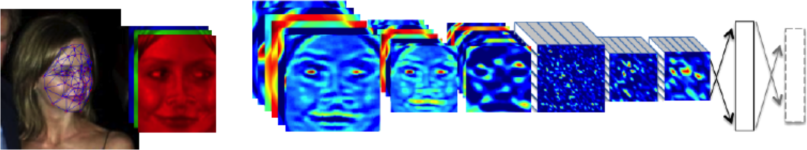
  • Example: face recognition

DeepFace

Outline of the DeepFace architecture. A front-end of a single convolution-pooling-convolution filtering on the rectified input, followed by three locally-connected layers and two fully-connected layers. Color illustrates feature maps produced at each layer. The net includes more than 120 million parameters, where more than 95% come from the local and fully connected.

Source: DeepFace (Taigman et al., 2014)

Deep Learning as Pinball

Uncertainty and Learning

  • In this “vanilla” form these machines “don’t know when they don’t know”.
  • Doubt is vital in real world decision making.
  • Incorporating this in systems is a long time focus of my technical research.

Comparison with Human Learning & Embodiment

  • The emulation of intelligence does not exhibit all the meta-modelling humans perform.

Data Science and Professionalisation

  • Industrial Revolution 4.0?
  • Industrial Revolution (1760-1840) term coined by Arnold Toynbee (1852-1883).
  • Maybe: But this one is dominated by data not capital
  • A revolution in information rather than energy.
  • That presents challenges and opportunities
  • Consider Apple vs Nokia: How you handle disruption.

compare digital oligarchy vs how Africa can benefit from the data revolution

A Time for Professionalisation?

  • New technologies historically led to new professions:
    • Brunel (born 1806): Civil, mechanical, naval
    • Tesla (born 1856): Electrical and power
    • William Shockley (born 1910): Electronic
    • Watts S. Humphrey (born 1927): Software

Why?

  • Codification of best practice.
  • Developing trust

Where are we?

  • Perhaps around the 1980s of programming.
    • We understand if, for, and procedures
    • But we don’t share best practice.
  • Let’s avoid the over formalisation of software engineering.

The Software Crisis

The major cause of the software crisis is that the machines have become several orders of magnitude more powerful! To put it quite bluntly: as long as there were no machines, programming was no problem at all; when we had a few weak computers, programming became a mild problem, and now we have gigantic computers, programming has become an equally gigantic problem.

Edsger Dijkstra (1930-2002), The Humble Programmer

The Data Crisis

The major cause of the data crisis is that machines have become more interconnected than ever before. Data access is therefore cheap, but data quality is often poor. What we need is cheap high-quality data. That implies that we develop processes for improving and verifying data quality that are efficient.

There would seem to be two ways for improving efficiency. Firstly, we should not duplicate work. Secondly, where possible we should automate work.

Me

Information Barons threaten our Privacy

{Our current information infrastructure bears a close relation with feudal systems of government. In the feudal system a lord had a duty of care over his serfs and vassals, a duty to protect subjects. But in practice there was a power-asymetry. In feudal days protection was against Viking raiders, today, it is against information raiders. However, when there is an information leak, when there is some failure in protections, it is already too late.

Alternatively, our data is publicly shared, as in an information commons. Akin to common land of the medieval village. But just as commons were subject to overgrazing and poor management, so it is that much of our data cannot be managed in this way. In particularly personal, sensitive data.

I explored this idea further in this .

Rest of the Talk

  • Importance of data infrastructure

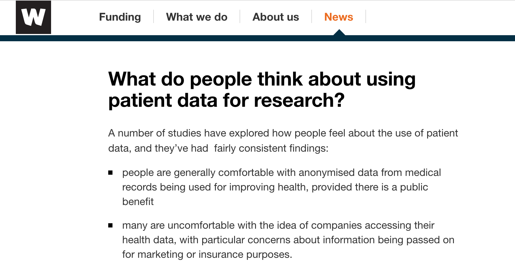
Understanding Patient Data
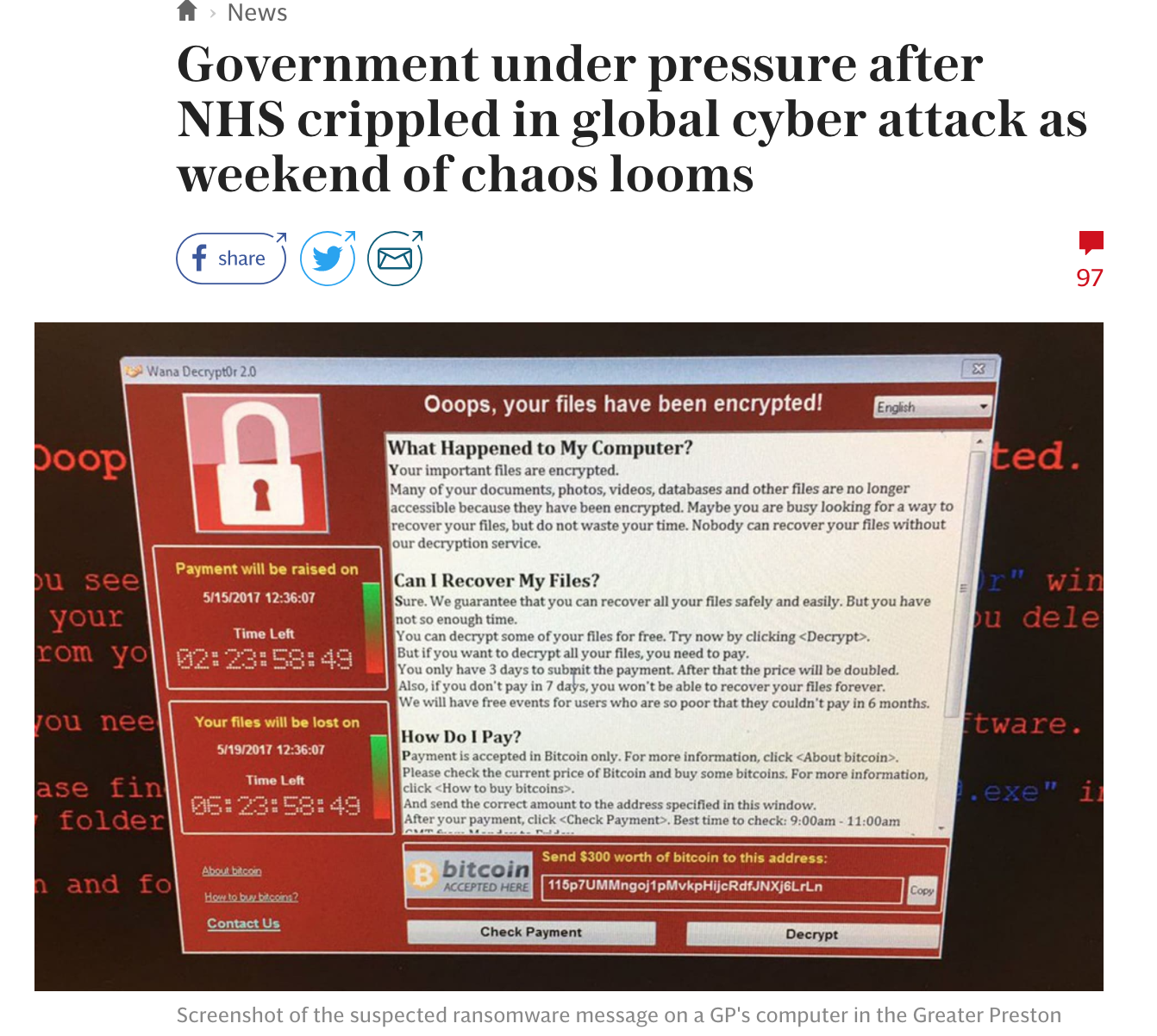
WannaCry

Bush Pilot Model

  • The difference between capability and intent.

Motivation

  1. Indsidious decision-making that has downstream instrumental effects we don’t control.
  2. A power-asymmetry between data-controllers and data-subjects
  3. A loss of personhood in the re-representation of ourselves in the digital world.
  4. The GDPR’s endeavour to curb contractual freedom cannot by itself reverse the power-asymmetry between data-controllers and data-subjects.

Analogy

  • Digital Democracy vs Digital Oligarchy Lawrence (2015a) or Information Feudalism Lawrence (2015b)
  • Data subjects, data controllers and data processors.

Thanks!

Delacroix, S., Lawrence, N.D., 2019. Bottom-up data trusts: Disturbing the “one size fits all” approach to data governance. International Data Privacy Law. https://doi.org/10.1093/idpl/ipz014

Edwards, L., 2004. The problem with privacy. International Review of Law Computers & Technology 18, 263–294.

Lawrence, N.D., 2017. Living together: Mind and machine intelligence. arXiv.

Lawrence, N.D., 2016. Data trusts could allay our privacy fears.

Lawrence, N.D., 2015a. Beware the rise of the digital oligarchy.

Lawrence, N.D., 2015b. The information barons threaten our autonomy and our privacy.

Taigman, Y., Yang, M., Ranzato, M., Wolf, L., 2014. DeepFace: Closing the gap to human-level performance in face verification, in: Proceedings of the IEEE Computer Society Conference on Computer Vision and Pattern Recognition. https://doi.org/10.1109/CVPR.2014.220