Data Science and the Professions
What is Machine Learning?
\[ \text{data} + \text{model} \xrightarrow{\text{compute}} \text{prediction}\]
- data : observations, could be actively or passively acquired (meta-data).
- model : assumptions, based on previous experience (other data! transfer learning etc), or beliefs about the regularities of the universe. Inductive bias.
- prediction : an action to be taken or a categorization or a quality score.
- Royal Society Report: Machine Learning: Power and Promise of Computers that Learn by Example
What is Machine Learning?
\[\text{data} + \text{model} \xrightarrow{\text{compute}} \text{prediction}\]
- To combine data with a model need:
- a prediction function \(\mappingFunction (\cdot)\) includes our beliefs about the regularities of the universe
- an objective function \(\errorFunction (\cdot)\) defines the cost of misprediction.
Machine Learning
- Driver of two different domains:
- Data Science: arises from the fact that we now capture data by happenstance.
- Artificial Intelligence: emulation of human behaviour.
- Connection: Internet of Things
Machine Learning
- Driver of two different domains:
- Data Science: arises from the fact that we now capture data by happenstance.
- Artificial Intelligence: emulation of human behaviour.
- Connection: Internet of
Things
Machine Learning
- Driver of two different domains:
- Data Science: arises from the fact that we now capture data by happenstance.
- Artificial Intelligence: emulation of human behaviour.
- Connection: Internet of People
What does Machine Learning do?
- ML Automates through Data
- Strongly related to statistics.
- Field underpins revolution in data science and AI
- With AI:
- logic, robotics, computer vision, speech
- With Data Science:
- databases, data mining, statistics, visualization
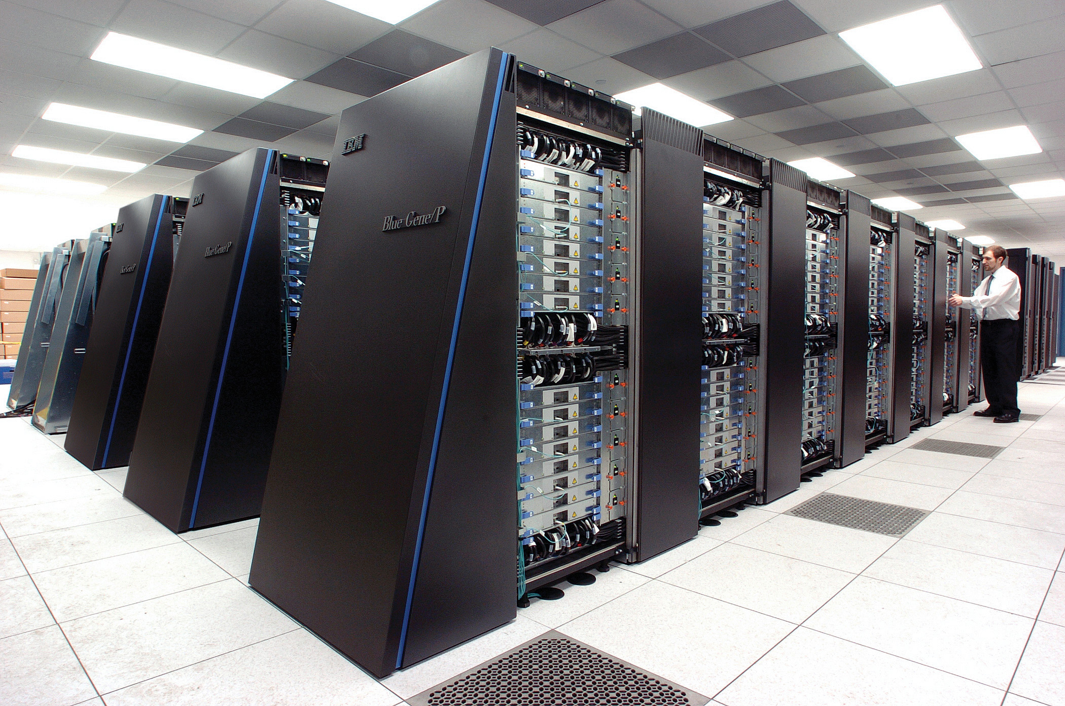
Embodiment Factors
|

|
|
| compute | \[\approx 100 \text{ gigaflops}\] | \[\approx 16 \text{ petaflops}\] |
| communicate | \[1 \text{ gigbit/s}\] | \[100 \text{ bit/s}\] |
| (compute/communicate) | \[10^{4}\] | \[10^{14}\] |
See “Living Together: Mind and Machine Intelligence” Lawrence (2017a)

.
Evolved Relationship
Evolved Relationship
What does Machine Learning do?
- Automation scales by codifying processes and automating them.
- Need:
- Interconnected components
- Compatible components
- Early examples:
- cf Colt 45, Ford Model T
Codify Through Mathematical Functions
- How does machine learning work?
- Jumper (jersey/sweater) purchase with logistic regression
\[ \text{odds} = \frac{p(\text{bought})}{p(\text{not bought})} \]
\[ \log \text{odds} = \beta_0 + \beta_1 \text{age} + \beta_2 \text{latitude}.\]
Codify Through Mathematical Functions
- How does machine learning work?
- Jumper (jersey/sweater) purchase with logistic regression
\[ p(\text{bought}) = \sigmoid{\beta_0 + \beta_1 \text{age} + \beta_2 \text{latitude}}.\]
Codify Through Mathematical Functions
- How does machine learning work?
- Jumper (jersey/sweater) purchase with logistic regression
\[ p(\text{bought}) = \sigmoid{\boldsymbol{\beta}^\top \inputVector}.\]
Codify Through Mathematical Functions
- How does machine learning work?
- Jumper (jersey/sweater) purchase with logistic regression
\[ \dataScalar = \mappingFunction\left(\inputVector, \boldsymbol{\beta}\right).\]
We call \(\mappingFunction(\cdot)\) the prediction function.
Fit to Data
- Use an objective function
\[\errorFunction(\boldsymbol{\beta}, \dataMatrix, \inputMatrix)\]
- E.g. least squares \[\errorFunction(\boldsymbol{\beta}, \dataMatrix, \inputMatrix) = \sum_{i=1}^\numData \left(\dataScalar_i - \mappingFunction(\inputVector_i, \boldsymbol{\beta})\right)^2.\]
Two Components
- Prediction function, \(\mappingFunction(\cdot)\)
- Objective function, \(\errorFunction(\cdot)\)
Deep Learning
- These are interpretable models: vital for disease etc.
- Modern machine learning methods are less interpretable
- Example: face recognition
Deep Learning
These are interpretable models: vital for disease modeling etc.
Modern machine learning methods are less interpretable
Example: face recognition
DeepFace
Outline of the DeepFace architecture. A front-end of a single convolution-pooling-convolution filtering on the rectified input, followed by three locally-connected layers and two fully-connected layers. Color illustrates feature maps produced at each layer. The net includes more than 120 million parameters, where more than 95% come from the local and fully connected.
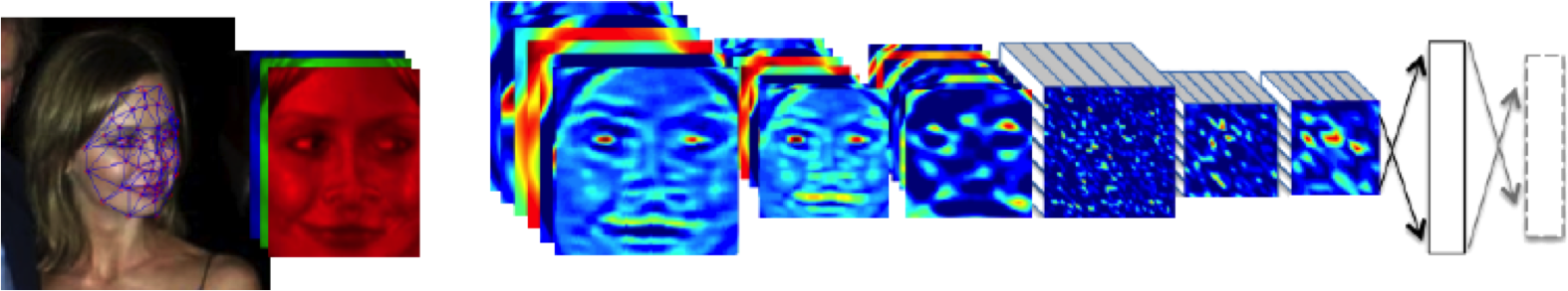
Source: DeepFace (Taigman et al., 2014)
Deep Learning as Pinball

Data Science and Professionalisation
- Industrial Revolution 4.0?
- Industrial Revolution (1760-1840) term coined by Arnold Toynbee (1852-1883).
- Maybe: But this one is dominated by data not capital
- A revolution in information rather than energy.
- That presents challenges and opportunities
- Consider Apple vs Nokia: How you handle disruption.
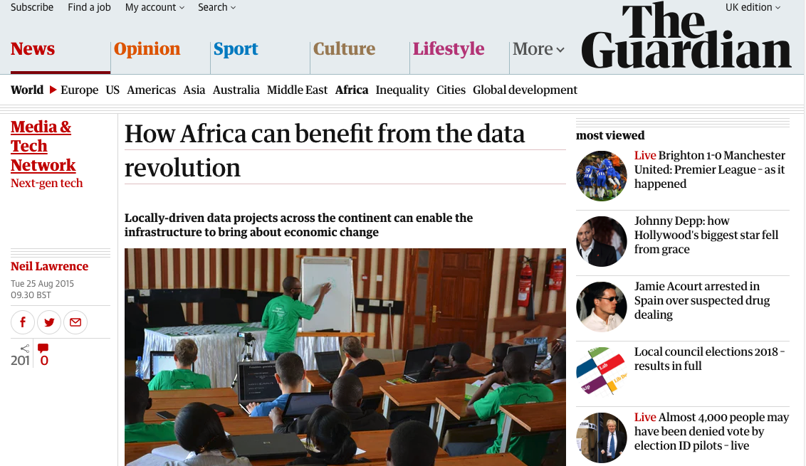
compare digital oligarchy vs how Africa can benefit from the data revolution
A Time for Professionalisation?
- New technologies historically led to new professions:
- Brunel (born 1806): Civil, mechanical, naval
- Tesla (born 1856): Electrical and power
- William Shockley (born 1910): Electronic
- Watts S. Humphrey (born 1927): Software
Why?
- Codification of best practice.
- Developing trust
Where are we?
- Perhaps around the 1980s of programming.
- We understand
if,for, and procedures - But we don’t share best practice.
- We understand
- Let’s avoid the over formalisation of software engineering.
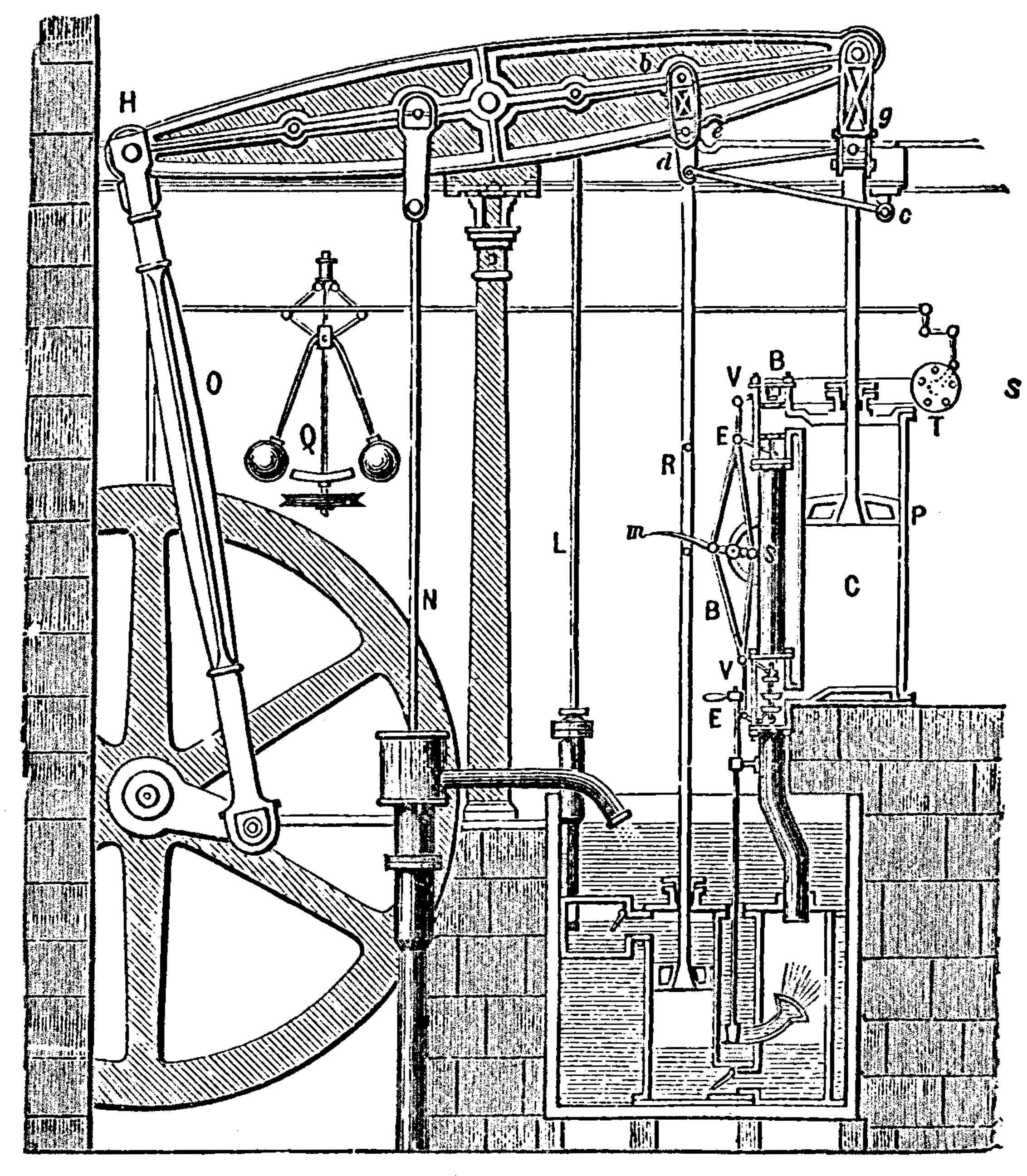
The Software Crisis
The major cause of the software crisis is that the machines have become several orders of magnitude more powerful! To put it quite bluntly: as long as there were no machines, programming was no problem at all; when we had a few weak computers, programming became a mild problem, and now we have gigantic computers, programming has become an equally gigantic problem.
Edsger Dijkstra (1930-2002), The Humble Programmer
The Data Crisis
The major cause of the data crisis is that machines have become more interconnected than ever before. Data access is therefore cheap, but data quality is often poor. What we need is cheap high-quality data. That implies that we develop processes for improving and verifying data quality that are efficient.
There would seem to be two ways for improving efficiency. Firstly, we should not duplicate work. Secondly, where possible we should automate work.
Me
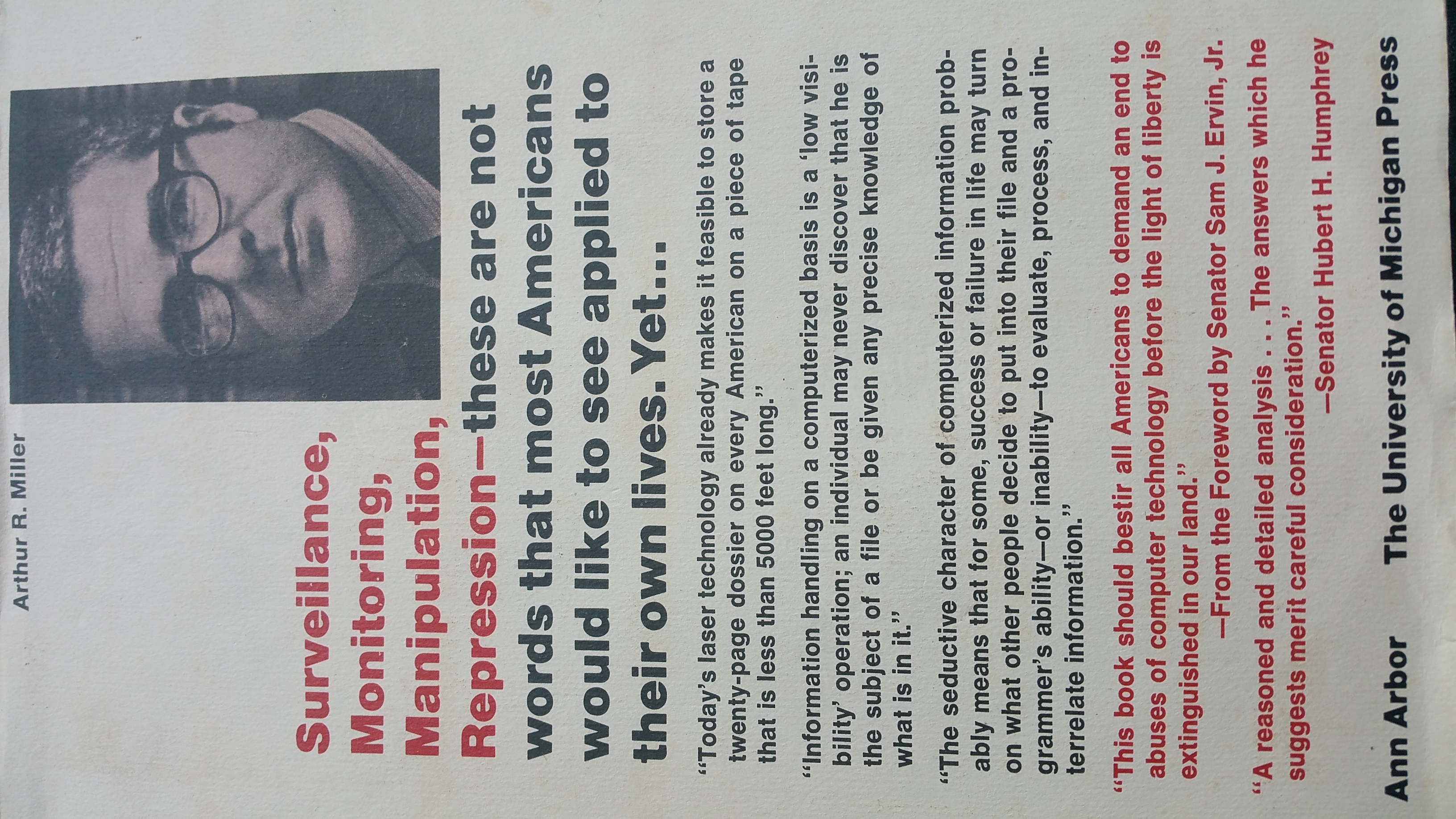
Power Asymmetries and Data
Privacy, Loss of Control and Marginalization
- Society is becoming harder to monitor
- Individual is becoming easier to monitor
Hate Speech or Political Dissent?
- social media monitoring for ‘hate speech’ can be easily turned to political dissent monitoring
Marketing
- can become more sinister when the target of the marketing is well understood and the (digital) environment of the target is also so well controlled
See .
Free Will
- What does it mean if a computer can predict our individual behavior better than we ourselves can?
Discrimination
- Potential for explicit and implicit discrimination on the basis of race, religion, sexuality, health status
- All prohibited under European law, but can pass unawares, or be implicit
- GDPR: General Data Protection Regulation
Discrimination
- Potential for explicit and implicit discrimination on the basis of race, religion, sexuality, health status
- All prohibited under European law, but can pass unawares, or be implicit
- GDPR: Good Data Practice Rules
Marginalization
- Credit scoring, insurance, medical treatment
- What if certain sectors of society are under-represented in our analysis?
- What if Silicon Valley develops everything for us?
Digital Revolution and Inequality?

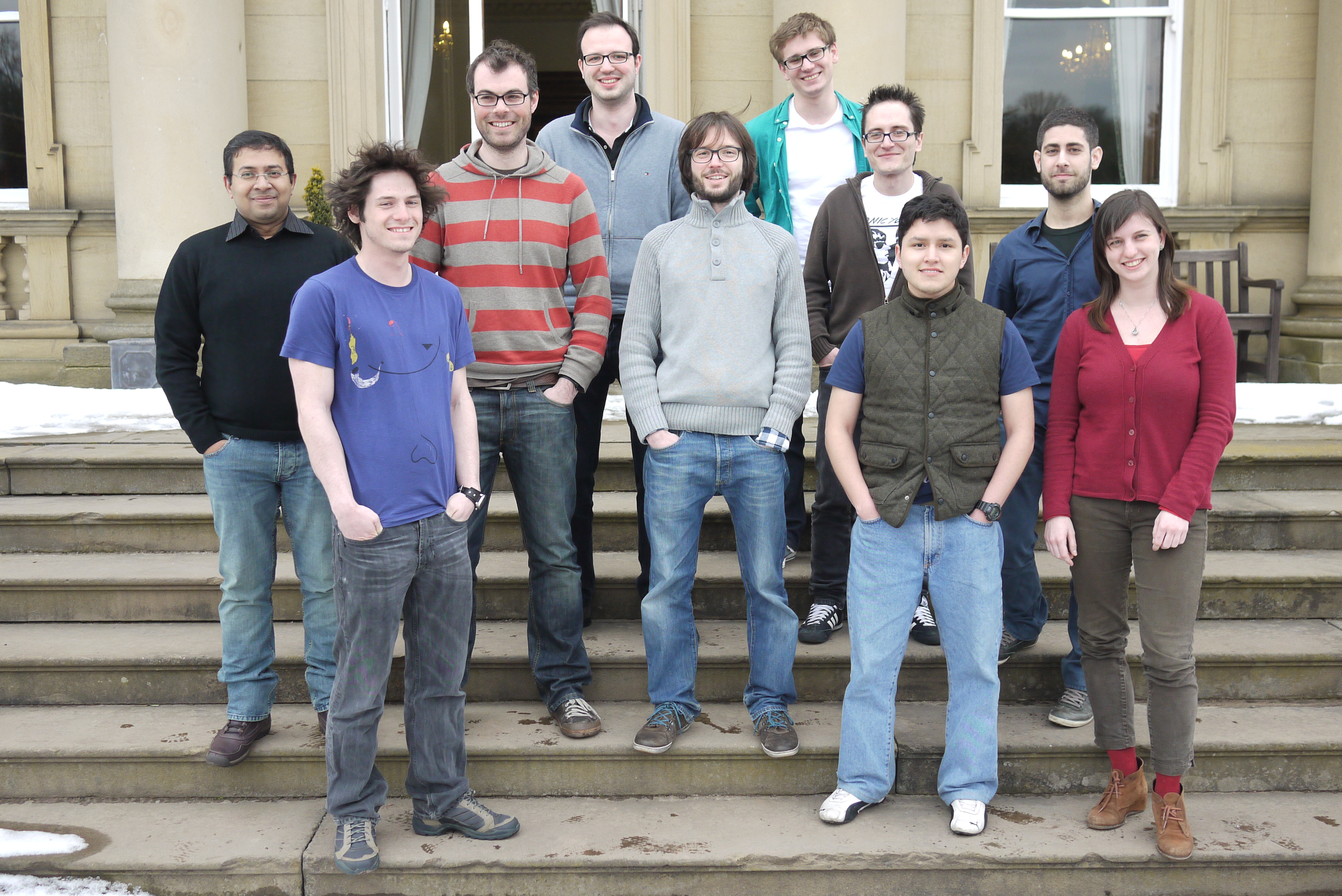
Data Science Africa is a bottom up initiative for capacity building in data science, machine learning and AI on the African continent
Example: Prediction of Malaria Incidence in Uganda
- Work with Ricardo Andrade Pacheco, John Quinn and Martin Mubaganzi (Makerere University, Uganda)
- See AI-DEV Group.
Malaria Prediction in Uganda
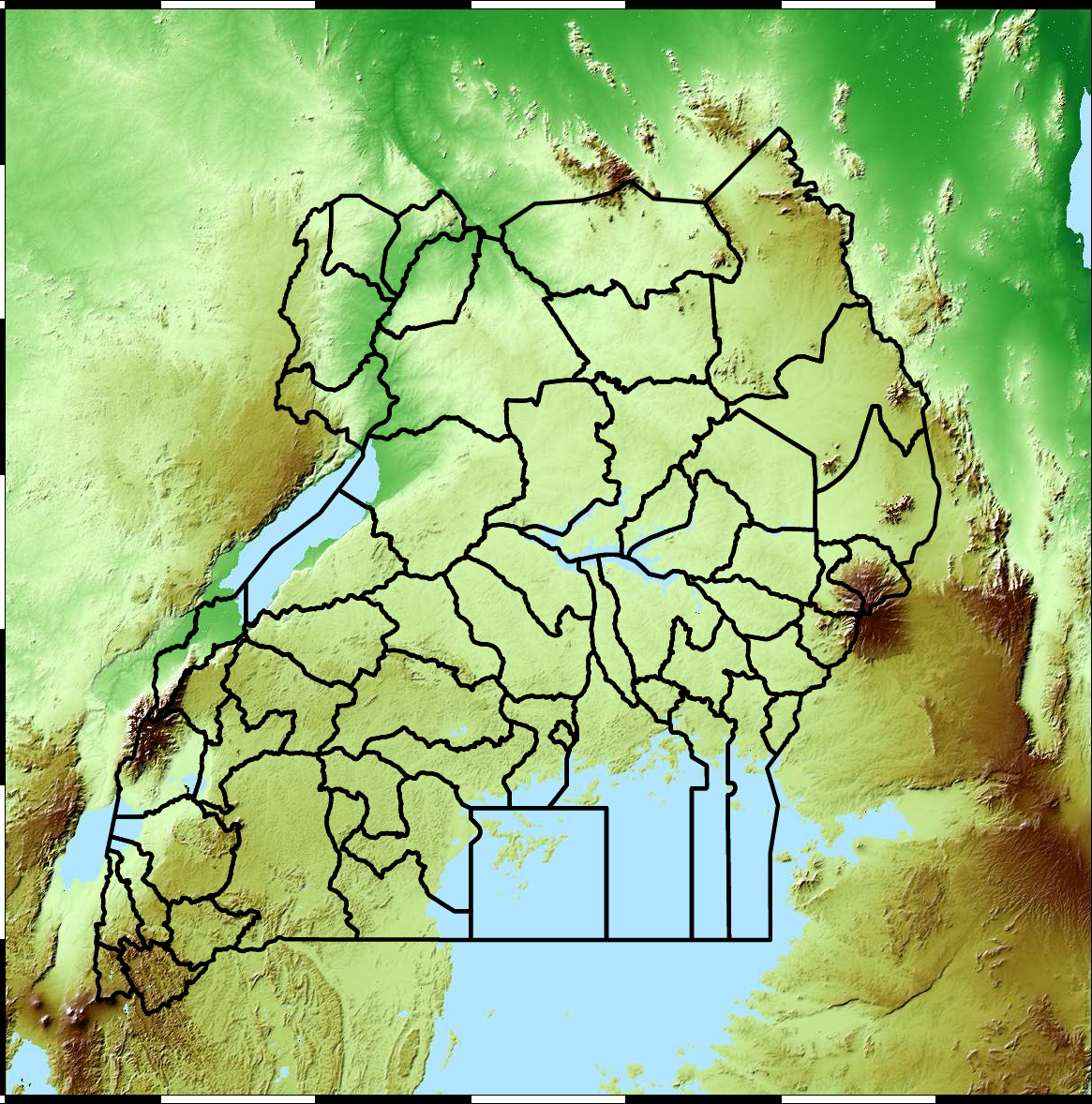
(Andrade-Pacheco et al., 2014; Mubangizi et al., 2014)
Tororo District
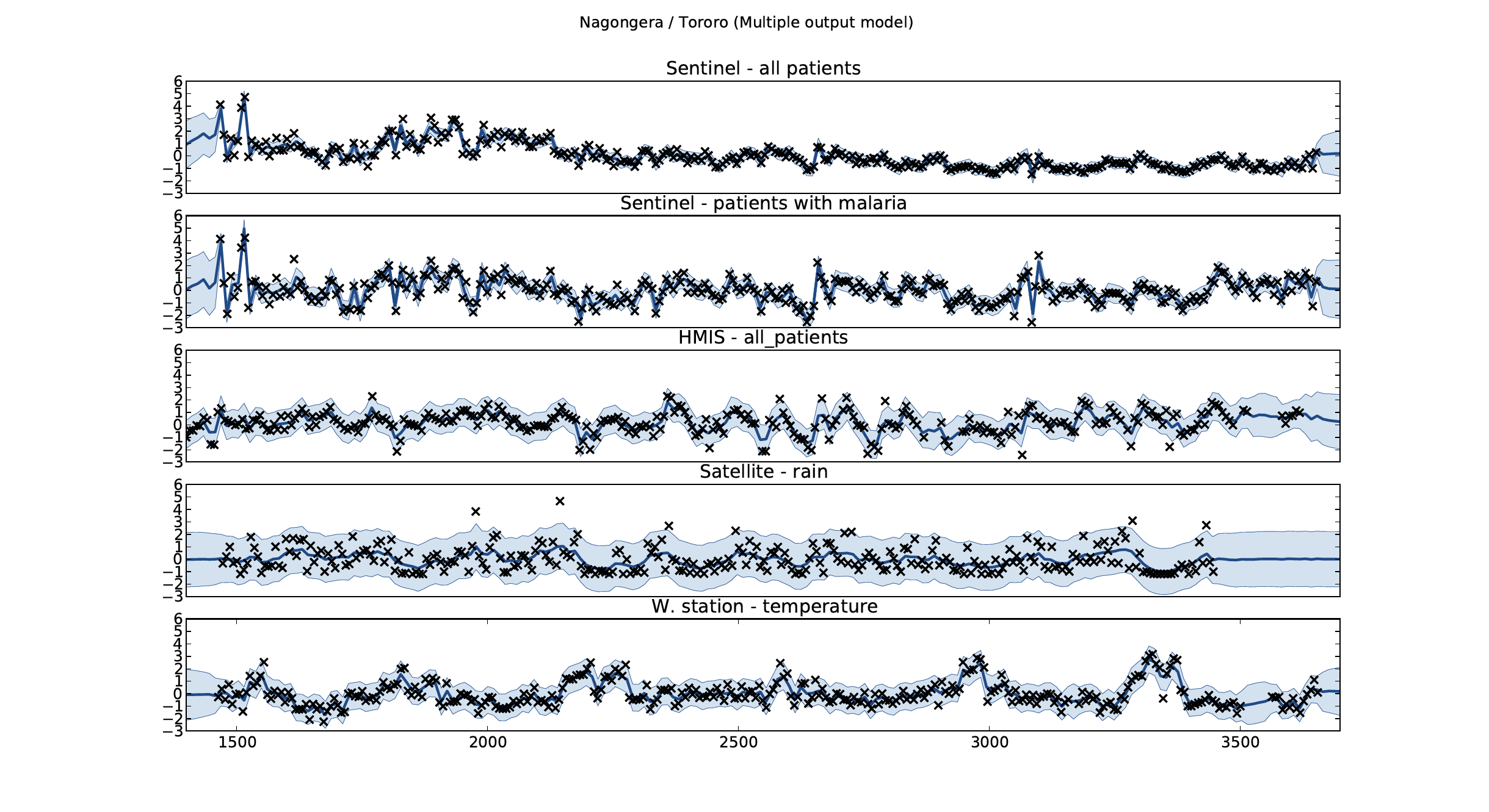
Malaria Prediction in Nagongera (Sentinel Site)
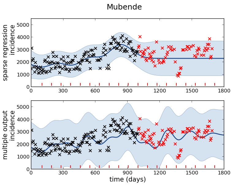
Mubende District
Malaria Prediction in Uganda
GP School at Makerere

Kabarole District
Early Warning System
Early Warning Systems
Motivation
- Indsidious decision-making that has downstream instrumental effects we don’t control.
- A power-asymmetry between data-controllers and data-subjects
- A loss of personhood in the re-representation of ourselves in the digital world.
- The GDPR’s endeavour to curb contractual freedom cannot by itself reverse the power-asymmetry between data-controllers and data-subjects.
Analogy
- Digital Democracy vs Digital Oligarchy Lawrence (2015a) or Information Feudalism Lawrence (2015b)
- Data subjects, data controllers and data processors.
Legal Mechanism of Trusts
- Fiduciary responsibility of Trustees.
- Burden of proof in negligence is reversed.
- Trustees are data controllers
- Beneficiaries are data subjects
- Power of data accumulation wielded on the beneficiaries behalf
- See Edwards (2004), Delacroix and Lawrence (2019) and Lawrence (2016)
Amelioration
- Work to ensure individual retains control of their own data
- We accept privacy in our real lives, need to accept it in our digital
- Control of persona and ability to project
- Need better technological solutions: trust and algorithms.
How GDPR May Help
Reflection on data eco-systems.
GDPR: Good Data Practice Rules
When viewed as best practice rather than regulation they hightlight problems in data ecosystems.

Rest of this Talk: Two Areas of Focus
- Reusability of Data
- Deployment of Machine Learning Systems
Data Readiness Levels
Data Readiness Levels
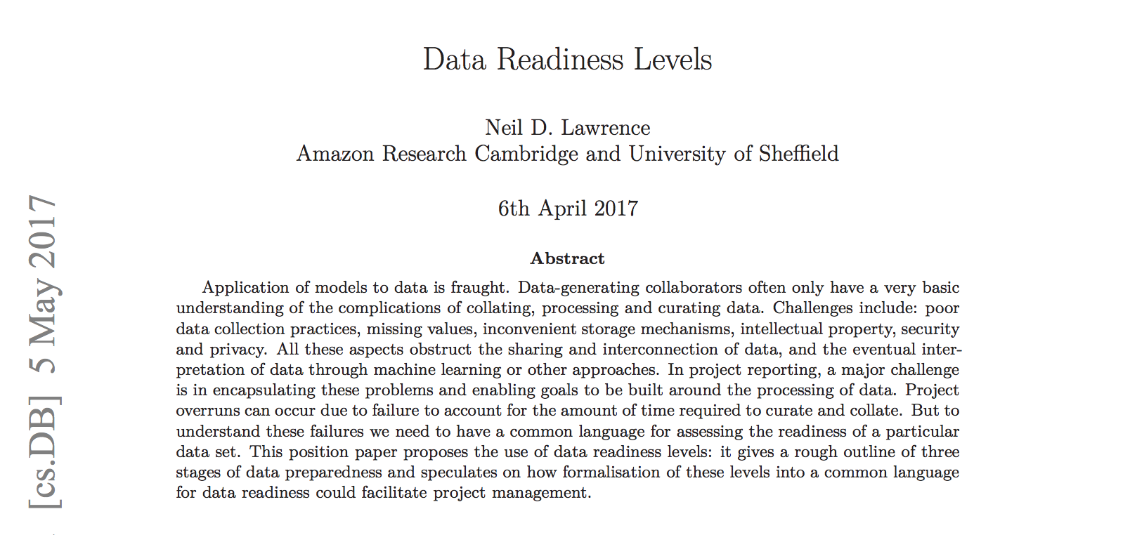
https://arxiv.org/pdf/1705.02245.pdf Data Readiness Levels (Lawrence, 2017b)
Three Grades of Data Readiness
- Grade C - accessibility
- Transition: data becomes electronically available
- Grade B - validity
- Transition: pose a question to the data.
- Grade A - usability
Accessibility: Grade C
- Hearsay data.
- Availability, is it actually being recorded?
- privacy or legal constraints on the accessibility of the recorded data, have ethical constraints been alleviated?
- Format: log books, PDF …
- limitations on access due to topology (e.g. it’s distributed across a number of devices)
- At the end of Grade C data is ready to be loaded into analysis software (R, SPSS, Matlab, Python, Mathematica)
Validity: Grade B
- faithfulness and representation
- visualisations.
- exploratory data analysis
- noise characterisation.
Grade B Checks
- Missing values.
- Schema alignment, record linkage, data fusion
- Example:
- Was a column or columns accidentally perturbed (e.g. through a sort operation that missed one or more columns)? Or was a gene name accidentally converted to a date?
Grade B Transition
- At the end of Grade B, ready to define a task, or question
- Compare with classical statistics:
- Classically: question is first data comes later.
- Today: data is first question comes later.
Data First
In a data first company teams own their data quality issues at least as far as grade B1.
Usability: Grade A
- The usability of data
- Grade A is about data in context.
- Consider appropriateness of a given data set to answer a particular question or to be subject to a particular analysis.
Recursive Effects
- Grade A may also require:
- data integration
- active collection of new data.
- rebalancing of data to ensure fairness
- annotation of data by human experts
- revisiting the collection (and running through the appropriate stages again)
A1 Data
- A1 data is ready to make available for challenges or AutoML platforms.
Contribute!
Also …
- Encourage greater interaction between application domains and data scientists
- Encourage visualization of data
See Also …
- Data Joel Tests
Deploying Artificial Intelligence
- Challenges in deploying AI.
- Currently this is in the form of “machine learning systems”
Internet of People
- Fog computing: barrier between cloud and device blurring.
- Computing on the Edge
- Complex feedback between algorithm and implementation
Deploying ML in Real World: Machine Learning Systems Design
- Major new challenge for systems designers.
- Internet of Intelligence but currently:
- AI systems are fragile
Machine Learning Systems Design
Fragility of AI Systems
- They are componentwise built from ML Capabilities.
- Each capability is independently constructed and verified.
- Pedestrian detection
- Road line detection
- Important for verification purposes.
Pigeonholing

Robust
- Need to move beyond pigeonholing tasks.
- Need new approaches to both the design of the individual components, and the combination of components within our AI systems.
Rapid Reimplementation
- Whole systems are being deployed.
- But they change their environment.
- The experience evolved adversarial behaviour.
Machine Learning Systems Design

Adversaries
- Stuxnet
- Mischevious-Adversarial
An Intelligent System
Joint work with M. Milo
An Intelligent System
Joint work with M. Milo
Peppercorns
- A new name for system failures which aren’t bugs.
- Difference between finding a fly in your soup vs a peppercorn in your soup.
Peppercorns
Turnaround And Update
- There is a massive need for turn around and update
- A redeploy of the entire system.
- This involves changing the way we design and deploy.
- Interface between security engineering and machine learning.
Conclusion
Artificial Intelligence and Data Science are fundamentally different.
In one you are dealing with data collected by happenstance.
In the other you are trying to build systems in the real world, often by actively collecting data.
Our approaches to systems design are building powerful machines that will be deployed in evolving environments.
Thanks!
- twitter: @lawrennd
- podcast: The Talking Machines
Guardian article on The data-driven economy will help marketers exploit us
Guardian article on How African can benefit from the data revolution
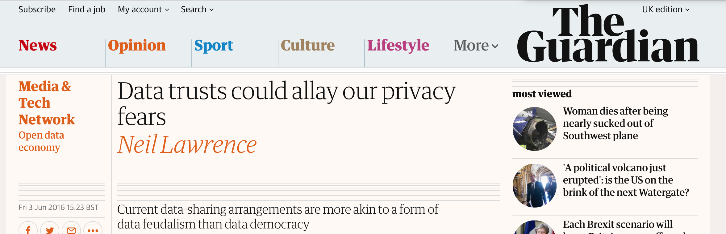
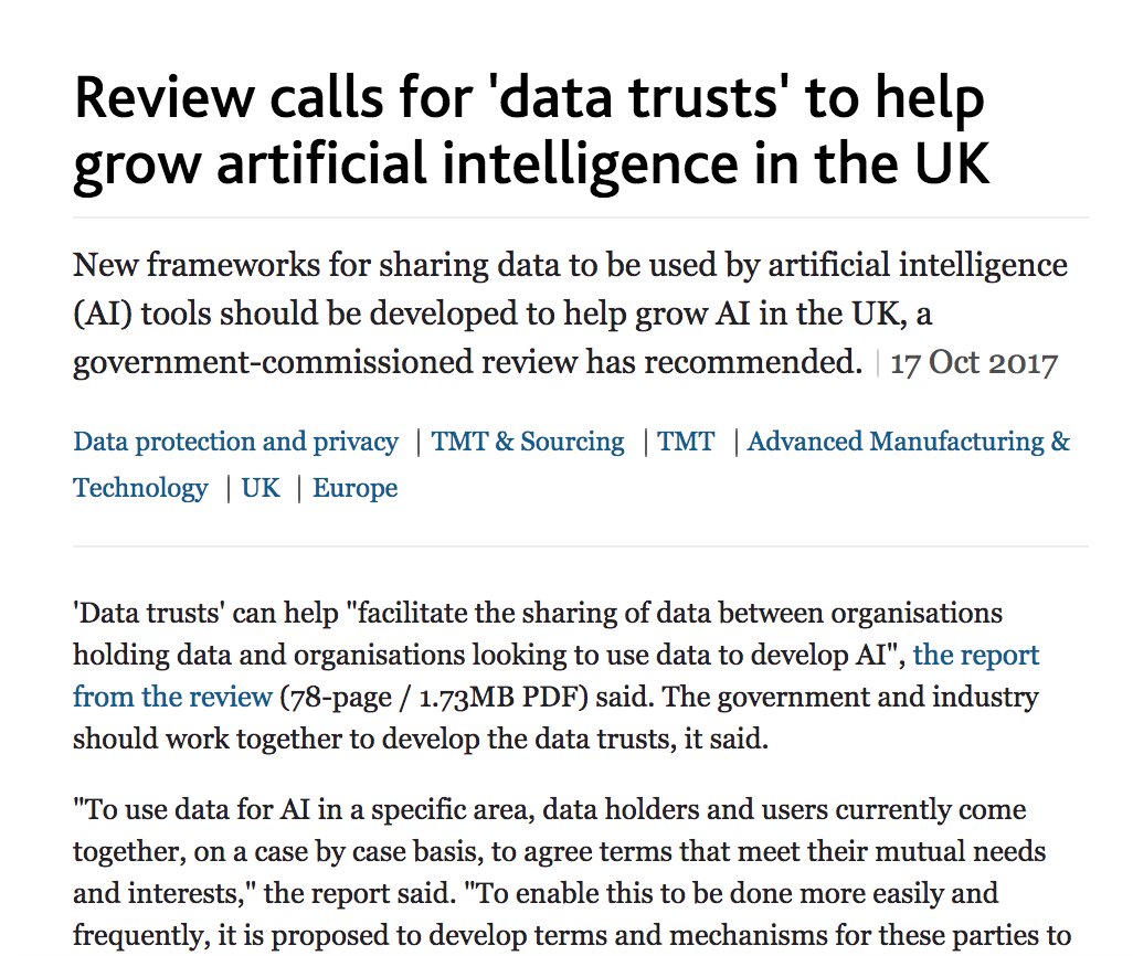
Guardian article on Data Trusts
Guardian article on Digital Oligarchies
Guardian article on Information Feudalism
Blog post on What is Machine Learning?
Blog post on System Zero
Blog post on Data Readiness Levels
Blog post on Decision Making and Diversity
Blog post on Natural vs Artifical Intelligence
References
Andrade-Pacheco, R., Mubangizi, M., Quinn, J., Lawrence, N.D., 2014. Consistent mapping of government malaria records across a changing territory delimitation. Malaria Journal 13. https://doi.org/10.1186/1475-2875-13-S1-P5
Delacroix, S., Lawrence, N.D., 2019. Bottom-up data trusts: Disturbing the “one size fits all” approach to data governance. International Data Privacy Law. https://doi.org/10.1093/idpl/ipz014
Edwards, L., 2004. The problem with privacy. International Review of Law Computers & Technology 18, 263–294.
Lawrence, N.D., 2017a. Living together: Mind and machine intelligence. arXiv.
Lawrence, N.D., 2017b. Data readiness levels. arXiv.
Lawrence, N.D., 2016. Data trusts could allay our privacy fears.
Lawrence, N.D., 2015a. Beware the rise of the digital oligarchy.
Lawrence, N.D., 2015b. The information barons threaten our autonomy and our privacy.
Mubangizi, M., Andrade-Pacheco, R., Smith, M.T., Quinn, J., Lawrence, N.D., 2014. Malaria surveillance with multiple data sources using Gaussian process models, in: 1st International Conference on the Use of Mobile ICT in Africa.
Taigman, Y., Yang, M., Ranzato, M., Wolf, L., 2014. DeepFace: Closing the gap to human-level performance in face verification, in: Proceedings of the IEEE Computer Society Conference on Computer Vision and Pattern Recognition. https://doi.org/10.1109/CVPR.2014.220