Data Science and Digital Systems

The Gartner Hype Cycle

Gartner Hype Cycle

❮ ❯

There are three types of lies: lies, damned lies and statistics

??

There are three types of lies: lies, damned lies and statistics

Benjamin Disraeli

There are three types of lies: lies, damned lies and statistics

Benjamin Disraeli 1804-1881

There are three types of lies: lies, damned lies and ‘big data’

Neil Lawrence 1972-?

Mathematical Statistics

‘Mathematical Data Science’

\[\text{data} + \text{model} \xrightarrow{\text{compute}} \text{prediction}\]

From Model to Decision

Artificial Intelligence and Data Science

• AI aims to equip computers with human capabilities
  • Image understanding
  • Computer vision
  • Speech recognition
  • Natural language understanding
  • Machine translation

Supervised Learning for AI

• Dominant approach today:
  • Generate large labelled data set from humans.
  • Use supervised learning to emulate that data.
    • E.g. ImageNet Russakovsky et al. (2015)
• Significant advances due to deep learning
  • E.g. Alexa, Amazon Go

Data Science

• Arises from happenstance data.
• Differs from statistics in that the question comes after data collection.

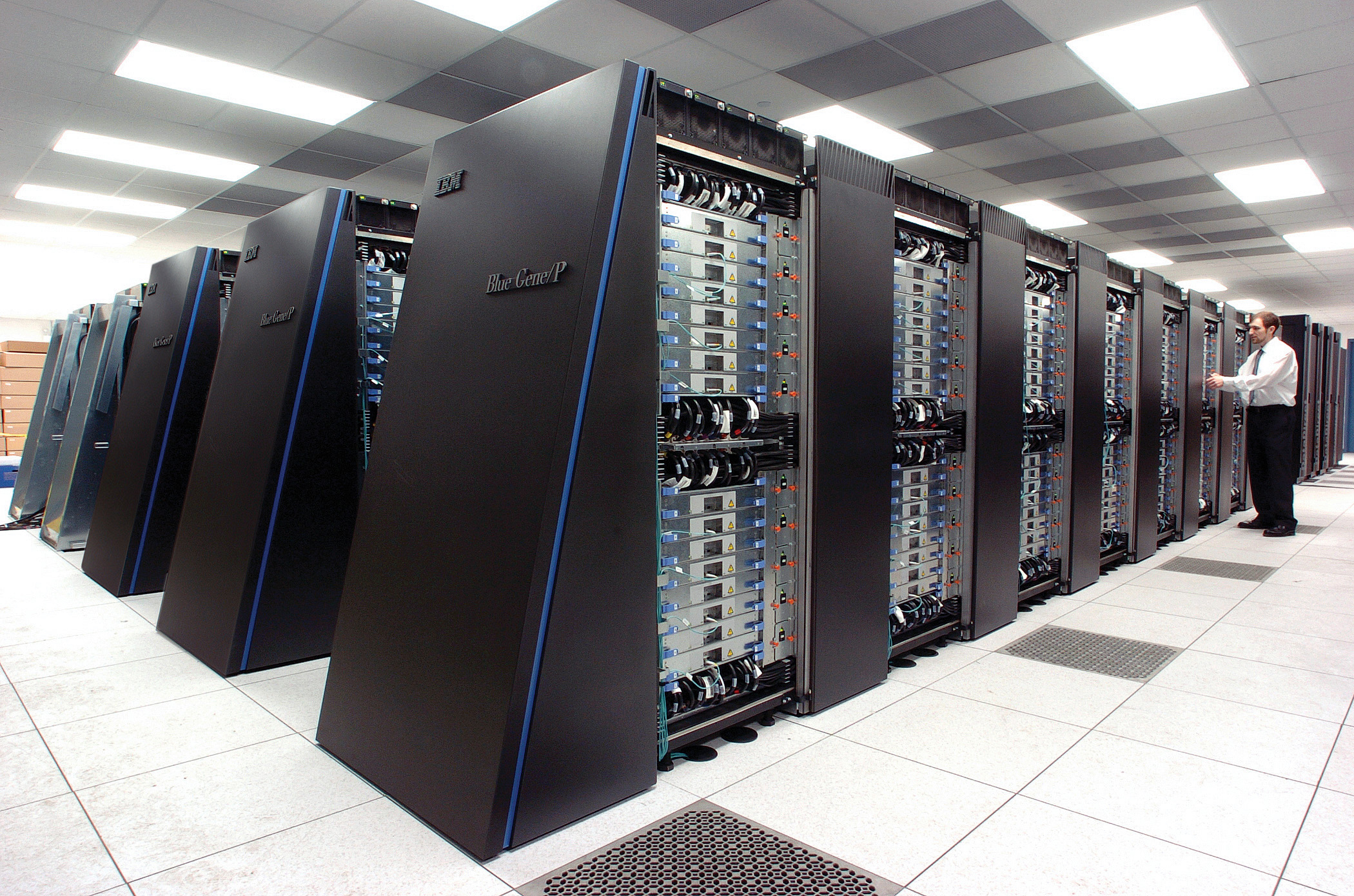
Embodiment Factors

compute	\[\approx 100 \text{ gigaflops}\]	\[\approx 16 \text{ petaflops}\]
communicate	\[1 \text{ gigbit/s}\]	\[100 \text{ bit/s}\]
(compute/communicate)	\[10^{4}\]	\[10^{14}\]

See “Living Together: Mind and Machine Intelligence” Lawrence (2017a)

.

Evolved Relationship

Evolved Relationship

Societal Effects

• This phenomenon has already revolutionised biology.
  • Large scale data acquisition and distribution.
  • Transcriptomics, genomics, epigenomics, ‘rich phenomics’.
• Great promise for personalized health.

Societal Effects

• Automated decision making within the computer based only on the data.
• Subjective biases need to be better understood.
• Particularly important where treatments are being prescribed.
  • Interventions could be far more subtle.

Societal Effects

• Shift in dynamic:
  • from direct human-data to indirect human-computer-data
  • modern data analysis is mediated by the machine
• This change of dynamics gives us the modern and emerging domain of data science

What does Machine Learning do?

• Automation scales by codifying processes and automating them.
• Need:
  • Interconnected components
  • Compatible components
• Early examples:
  • cf Colt 45, Ford Model T

Codify Through Mathematical Functions

• How does machine learning work?
• Jumper (jersey/sweater) purchase with logistic regression

\[ \text{odds} = \frac{p(\text{bought})}{p(\text{not bought})} \]

\[ \log \text{odds} = \beta_0 + \beta_1 \text{age} + \beta_2 \text{latitude}.\]

Codify Through Mathematical Functions

• How does machine learning work?
• Jumper (jersey/sweater) purchase with logistic regression

\[ p(\text{bought}) = \sigmoid{\beta_0 + \beta_1 \text{age} + \beta_2 \text{latitude}}.\]

Codify Through Mathematical Functions

• How does machine learning work?
• Jumper (jersey/sweater) purchase with logistic regression

\[ p(\text{bought}) = \sigmoid{\boldsymbol{\beta}^\top \inputVector}.\]

Codify Through Mathematical Functions

• How does machine learning work?
• Jumper (jersey/sweater) purchase with logistic regression

\[ \dataScalar = \mappingFunction\left(\inputVector, \boldsymbol{\beta}\right).\]

Fit to Data

• Use an objective function

\[\errorFunction(\boldsymbol{\beta}, \dataMatrix, \inputMatrix)\]

Two Components

• Prediction function, \(\mappingFunction(\cdot)\)
• Objective function, \(\errorFunction(\cdot)\)

Deep Learning

• These are interpretable models: vital for disease modeling etc.

• Modern machine learning methods are less interpretable

• Example: face recognition

DeepFace

Outline of the DeepFace architecture. A front-end of a single convolution-pooling-convolution filtering on the rectified input, followed by three locally-connected layers and two fully-connected layers. Color illustrates feature maps produced at each layer. The net includes more than 120 million parameters, where more than 95% come from the local and fully connected.

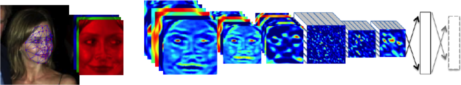
Source: DeepFace (Taigman et al., 2014)

Deep Learning as Pinball

Data Science and Professionalisation

• Industrial Revolution 4.0?
• Industrial Revolution (1760-1840) term coined by Arnold Toynbee (1852-1883).
• Maybe: But this one is dominated by data not capital
• A revolution in information rather than energy.
• That presents challenges and opportunities
• Consider Apple vs Nokia: How you handle disruption.

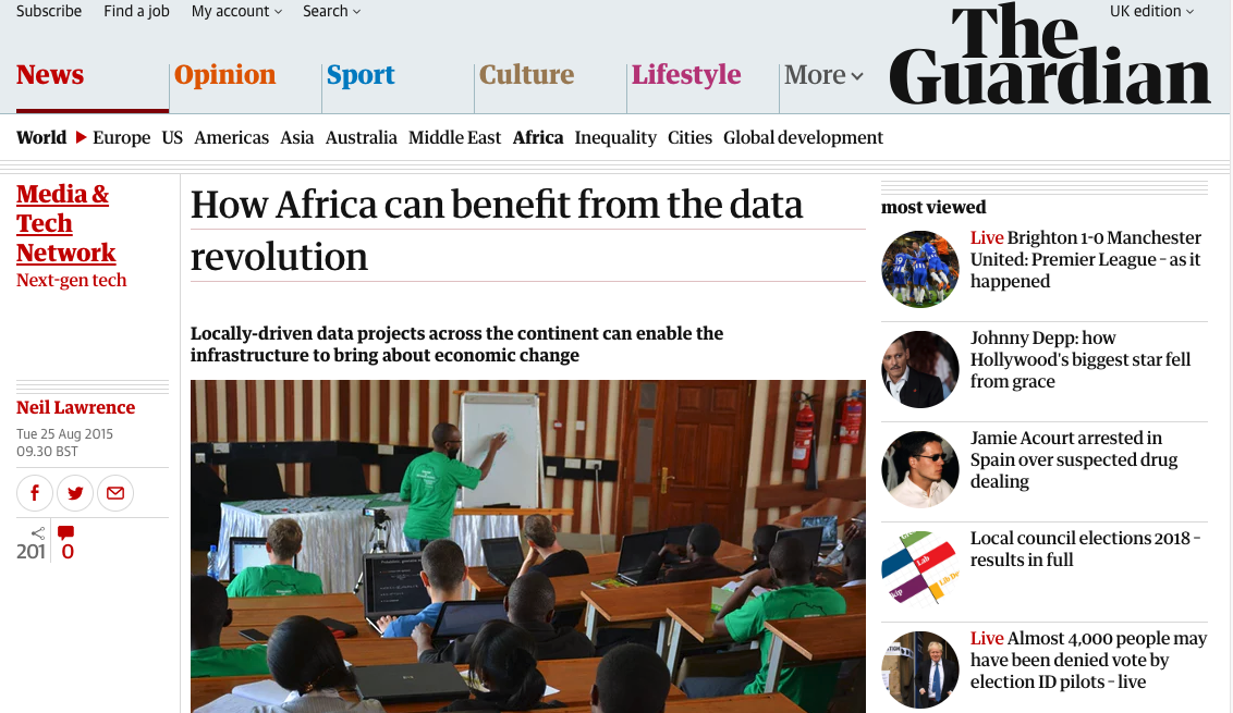
compare digital oligarchy vs how Africa can benefit from the data revolution

A Time for Professionalisation?

• New technologies historically led to new professions:
  • Brunel (born 1806): Civil, mechanical, naval
  • Tesla (born 1856): Electrical and power
  • William Shockley (born 1910): Electronic
  • Watts S. Humphrey (born 1927): Software

Why?

• Codification of best practice.
• Developing trust

Where are we?

• Perhaps around the 1980s of programming.
  • We understand if, for, and procedures
  • But we don’t share best practice.
• Let’s avoid the over formalisation of software engineering.

Thoughts from Willis’s Talk

• Analytics: Data Science for Business Graduates
• We are entering a golden era for statistics.
• To take advantage:
  • Statisticians need to learn to scale.
  • Statisticians need to learn to code (properly!).
• Can do attitude vs Can’t do attitude.

Challenges

1. Paradoxes of the Data Society

2. Quantifying the Value of Data

3. Privacy, loss of control, marginalization

Breadth or Depth Paradox

The Paradox of Measurement

• Able to quantify to a greater and greater degree the actions of individuals

• But less able to characterize society

• As we measure more, we understand less

What?

• Perhaps greater preponderance of data is making society itself more complex
• Therefore traditional approaches to measurement are failing
• Curate’s egg of a society: it is only ‘measured in parts’

Breadth vs Depth

• Modern Measurement deals with depth (many subjects) … or breadth lots of detail about subject.
• Can deal with large or large
• But what about
  • roughly equal to ?
  • Stratification of populations: batch effects etc.

Wood or Tree

• Can either see a wood or a tree.
  

Examples

• Election polls (UK 2015 elections, EU referendum, US 2016 elections)
• Clinical trials vs personalized medicine: Obtaining statistical power where interventions are subtle. e.g. social media

Challenges

• Social media memes
• Filter bubbles and echo chambers

Solutions

• More classical statistics!
  • Like the ‘paperless office’
• A better characterization of human needs and flaws
• Larger studies (100,000 genome)

Quantifying the Value of Data

There’s a sea of data, but most of it is undrinkable.

We require data-desalination before it can be consumed!

Data

• 90% of our time is spent on validation and integration (Leo Anthony Celi)
• “The Dirty Work We Don’t Want to Think About” (Eric Xing)
• “Voodoo to get it decompressed” (Francisco Giminez)
• In health care clinicians collect the data and often control the direction of research through guardianship of data.

Value

• How do we measure value in the data economy?
• How do we encourage data workers: curation and management
  • Incentivization for sharing and production.
  • Quantifying the value in the contribution of each actor.

Credit Allocation

• Direct work on data generates an enormous amount of ‘value’ in the data economy but this is unaccounted in the economy

• Hard because data is difficult to ‘embody’

• Value of shared data: Wellcome Trust 2010 Joint Statement (from the “Foggy Bottom” meeting)

Data Readiness Levels

Data Readiness Levels

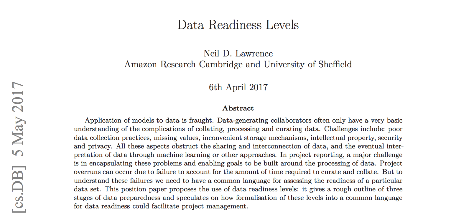
https://arxiv.org/pdf/1705.02245.pdf Data Readiness Levels (Lawrence, 2017b)

Three Grades of Data Readiness

• Grade C - accessibility
  • Transition: data becomes electronically available
• Grade B - validity
  • Transition: pose a question to the data.
• Grade A - usability

Accessibility: Grade C

• Hearsay data.
• Availability, is it actually being recorded?
• privacy or legal constraints on the accessibility of the recorded data, have ethical constraints been alleviated?
• Format: log books, PDF …
• limitations on access due to topology (e.g. it’s distributed across a number of devices)
• At the end of Grade C data is ready to be loaded into analysis software (R, SPSS, Matlab, Python, Mathematica)

Validity: Grade B

• faithfulness and representation
• visualisations.
• exploratory data analysis
• noise characterisation.

Grade B Checks

• Missing values.
• Schema alignment, record linkage, data fusion
• Example:
  • Was a column or columns accidentally perturbed (e.g. through a sort operation that missed one or more columns)? Or was a gene name accidentally converted to a date?

Grade B Transition

• At the end of Grade B, ready to define a task, or question
• Compare with classical statistics:
  • Classically: question is first data comes later.
  • Today: data is first question comes later.

Data First

In a data first company teams own their data quality issues at least as far as grade B1.

Usability: Grade A

• The usability of data
  • Grade A is about data in context.
• Consider appropriateness of a given data set to answer a particular question or to be subject to a particular analysis.

Recursive Effects

• Grade A may also require:
  • data integration
  • active collection of new data.
  • rebalancing of data to ensure fairness
  • annotation of data by human experts
  • revisiting the collection (and running through the appropriate stages again)

A1 Data

• A1 data is ready to make available for challenges or AutoML platforms.

Contribute!

Also …

• Encourage greater interaction between application domains and data scientists
• Encourage visualization of data

See Also …

• Data Joel Tests
  • proposal by Damon Civin and
  • proposal by Nick Elprin

Solutions

• Encourage greater interaction between application domains and data scientists
• Encourage visualization of data
• Adoption of ‘data readiness levels’
• Implications for incentivization schemes

Privacy, Loss of Control and Marginalization

• Society is becoming harder to monitor
• Individual is becoming easier to monitor

Hate Speech or Political Dissent?

• social media monitoring for ‘hate speech’ can be easily turned to political dissent monitoring

Marketing

• can become more sinister when the target of the marketing is well understood and the (digital) environment of the target is also so well controlled

See .

Free Will

• What does it mean if a computer can predict our individual behavior better than we ourselves can?

Discrimination

• Potential for explicit and implicit discrimination on the basis of race, religion, sexuality, health status
• All prohibited under European law, but can pass unawares, or be implicit
• GDPR: General Data Protection Regulation

Discrimination

• Potential for explicit and implicit discrimination on the basis of race, religion, sexuality, health status
• All prohibited under European law, but can pass unawares, or be implicit
• GDPR: Good Data Practice Rules

Marginalization

• Credit scoring, insurance, medical treatment
• What if certain sectors of society are under-represented in our analysis?
• What if Silicon Valley develops everything for us?

Digital Revolution and Inequality?

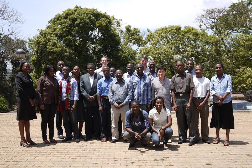
Data Science Africa is a bottom up initiative for capacity building in data science, machine learning and AI on the African continent

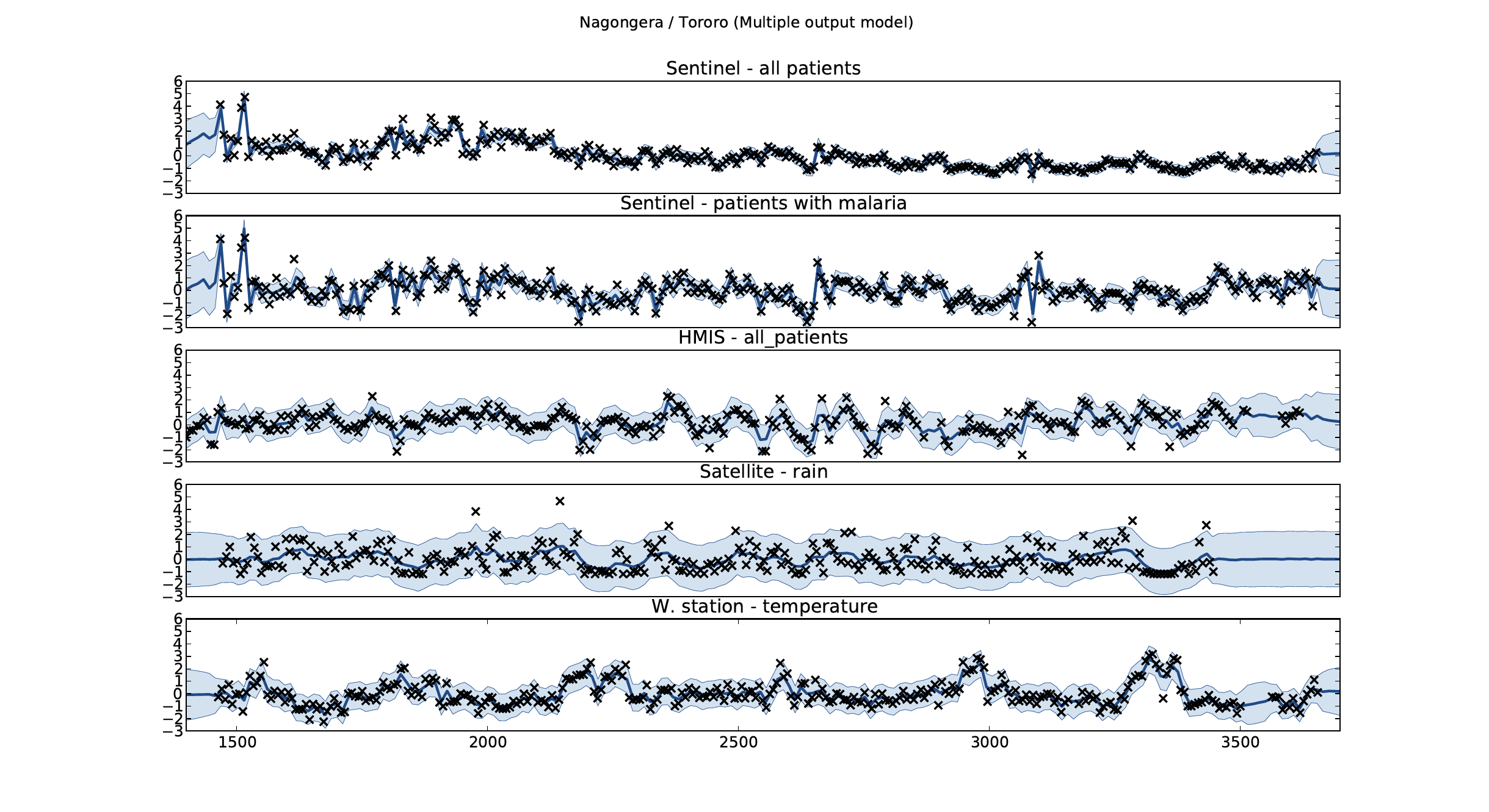
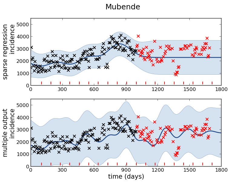
Example: Prediction of Malaria Incidence in Uganda

• Work with Ricardo Andrade Pacheco, John Quinn and Martin Mubaganzi (Makerere University, Uganda)
• See AI-DEV Group.

Malaria Prediction in Uganda

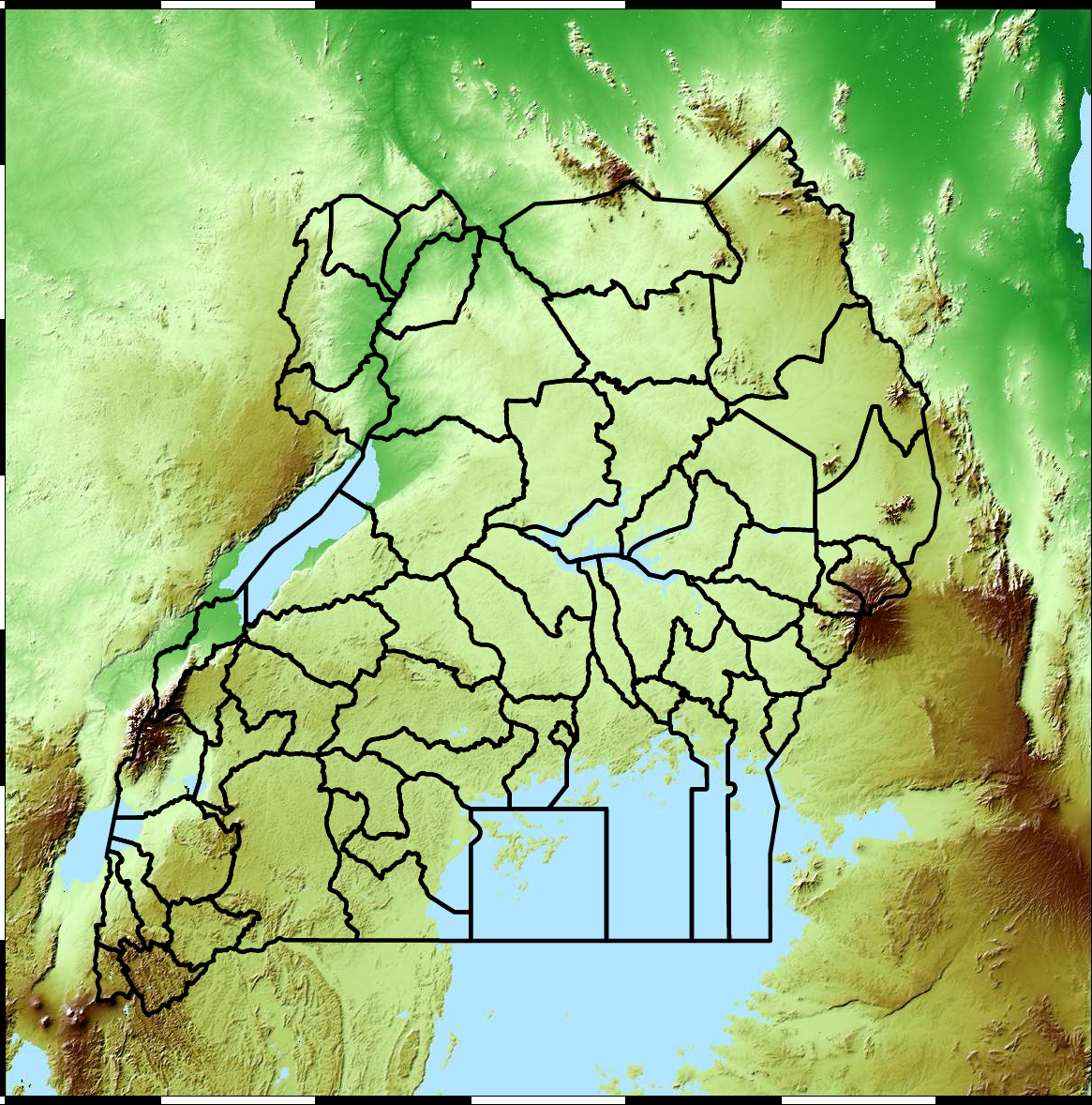
(Andrade-Pacheco et al., 2014; Mubangizi et al., 2014)

Tororo District

Malaria Prediction in Nagongera (Sentinel Site)

Mubende District

Malaria Prediction in Uganda

GP School at Makerere

Kabarole District

Early Warning System

Early Warning Systems

Motivation

1. Indsidious decision-making that has downstream instrumental effects we don’t control.
2. A power-asymmetry between data-controllers and data-subjects
3. A loss of personhood in the re-representation of ourselves in the digital world.
4. The GDPR’s endeavour to curb contractual freedom cannot by itself reverse the power-asymmetry between data-controllers and data-subjects.

Analogy

• Digital Democracy vs Digital Oligarchy Lawrence (2015a) or Information Feudalism Lawrence (2015b)
• Data subjects, data controllers and data processors.

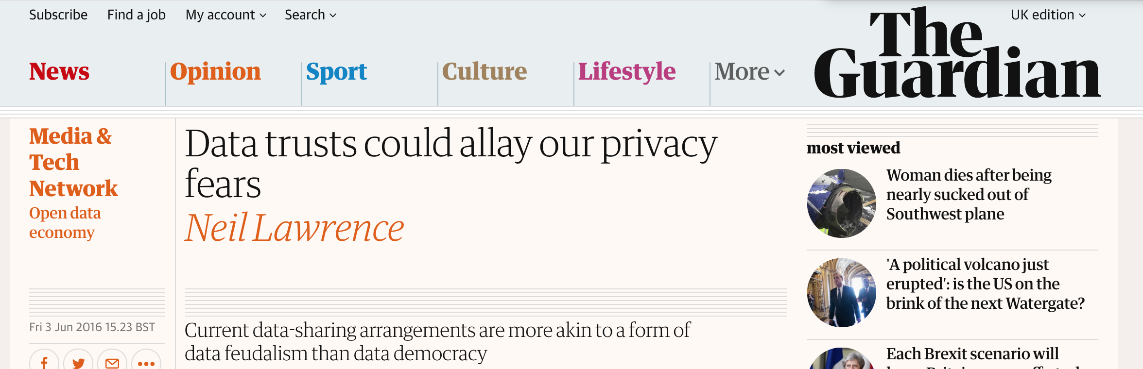
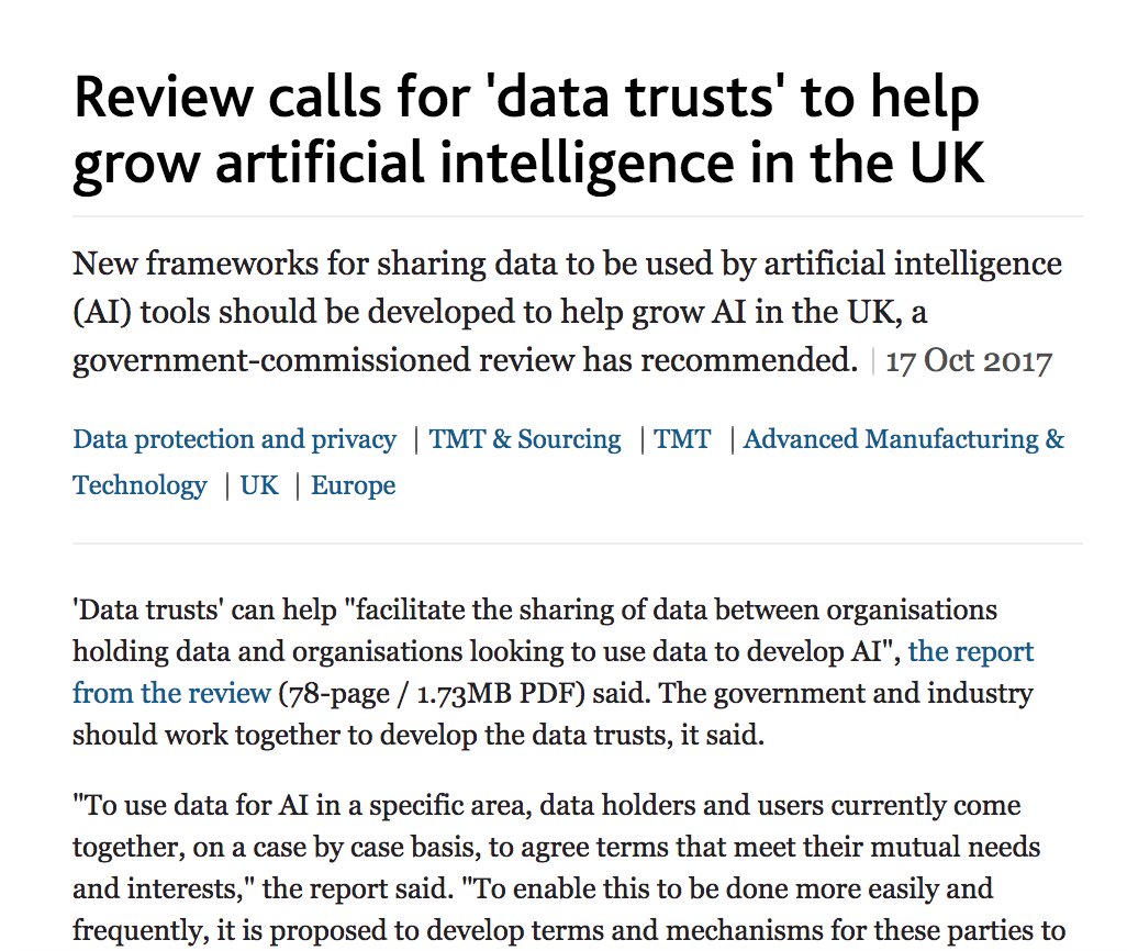
Legal Mechanism of Trusts

• Fiduciary responsibility of Trustees.
  • Burden of proof in negligence is reversed.
• Trustees are data controllers
• Beneficiaries are data subjects
• Power of data accumulation wielded on the beneficiaries behalf
• See Edwards (2004), Delacroix and Lawrence (2019) and Lawrence (2016)

Amelioration

• Work to ensure individual retains control of their own data
• We accept privacy in our real lives, need to accept it in our digital
• Control of persona and ability to project
• Need better technological solutions: trust and algorithms.

You can also check this

.

Amazon: Bits and Atoms

Artificial Intelligence

• Challenges in deploying AI.
• Currently this is in the form of “machine learning systems”

Internet of People

• Fog computing: barrier between cloud and device blurring.
  • Computing on the Edge
• Complex feedback between algorithm and implementation

Deploying ML in Real World: Machine Learning Systems Design

• Major new challenge for systems designers.
• Internet of Intelligence but currently:
  • AI systems are fragile

Supply Chain

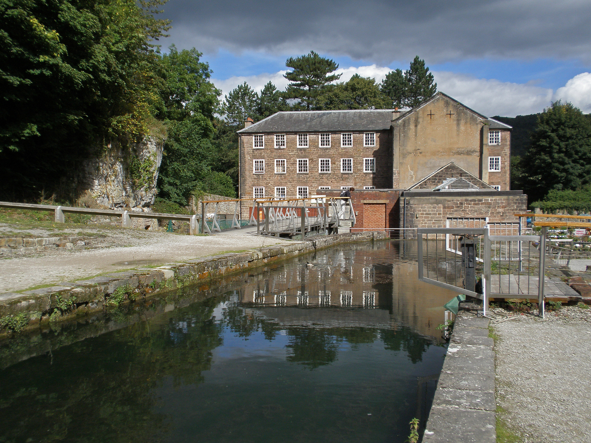
Cromford

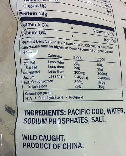
Deep Freeze

Deep Freeze

Machine Learning in Supply Chain

• Supply chain: Large Automated Decision Making Network
• Major Challenge:
  • We have a mechanistic understanding of supply chain.
  • Machine learning is a data driven technology.

The Tribal Mentality

• \(\text{data} + \text{model}\) is not new.
  • Dates back to Newton, Laplace, Gauss
• Plethora of fields: E.g.
  • Operations Research
  • Control
  • Econometrics
  • Statistics
  • Machine learning
  • Data science

The Tribal Mentality

• This can lead to confusion:
  • Different academic fields are:
    • Born in different eras
    • Driven by different motivations
    • Arrive at different solutions

Tribalism Can be Good

• Allows for consensus on best practice.
• Shared set of goals
• Ease of commiunication
• Rapid deployment of robust solutions

Professional Tribes

• This is the nature of professions
  • lawyers
  • medics
  • doctors
  • engineers
  • accountants

Different Views

\[\text{data} + \text{model}\]

• For OR, control, stats etc.
• More things unite us rather than divide us.

We’re no longer hunter gatherers …

• The automation challenges we face require
  • all of our best ideas.
  • rethinking what \(\text{data}+\text{model}\) means
  • rapid deployment and continuous monitoring
• This is the era of data science

Discomfort and Disconformation

• Talking across field boundaries is critical.
• It helps us disconfirm our beliefs.
• It’s not comfortable, but it’s vital.

THE THREE Ds of ML SYSTEMS DESIGN

The Three Ds of Machine Learning Systems Design

• Three primary challenges of Machine Learning Systems Design.

1. Decomposition
2. Data
3. Deployment

Decomposition

• ML is not Magical Pixie Dust.
• It cannot be sprinkled thoughtlessly.
• We cannot simply automate all decisions through data

Decomposition

We are constrained by:

1. Our data.
2. The models.

Decomposition of Task

• Careful thought needs to be put into sub-processes of task.
• Any repetitive task is a candidate for automation.

Pigeonholing

Pigeonholing

1. Can we decompose decision we need to repetitive sub-tasks where inputs and outputs are well defined?
2. Are those repetitive sub-tasks well represent by a mathematical mapping?

A Trap

• Over emphasis on the type of model we’re deploying.
• Under emphasis on the appropriateness of the task decomposition.

Chicken and Egg

Co-evolution

• Absolute decomposition is impossible.
• If we deploy a weak component in one place, downstream system will compensate.
• Systems co-evolve … there is no simple solution
• Trade off between performance and decomposability.
  • Need to monitor deployment

Data

• Hard to overstate its importance.
• Half the equation of \(\text{data} + \text{model}\).
• Often utterly neglected.

Data Neglect

• Arises for two reasons.
  1. Data cleaning is perceived as tedious.
  2. Data cleaning is complex.

Data Cleaning

• Seems difficult to formulate into readily teachable princples.
• Heavily neglected in data science, statistics and ML courses.
• In practice most scientists spend around 80% of time data cleaning.

The Software Crisis

The Data Crisis

The major cause of the data crisis is that machines have become more interconnected than ever before. Data access is therefore cheap, but data quality is often poor. What we need is cheap high-quality data. That implies that we develop processes for improving and verifying data quality that are efficient.

There would seem to be two ways for improving efficiency. Firstly, we should not duplicate work. Secondly, where possible we should automate work.

Me

Data Science as Debugging

• Analogies: For Software Engineers describe data science as debugging.

80/20 in Data Science

• Anecdotally for a given challenge
  • 80% of time is spent on data wrangling.
  • 20% of time spent on modelling.
• Many companies employ ML Engineers focussing on models not data.

Deployment

Premise

Our machine learning is based on a software systems view that is 20 years out of date.

Continuous Deployment

• Deployment of modeling code.
• Data dependent models in production need continuous monitoring.
• Continous monitoring implies statistical tests rather than classic software tests.

Continuous Monitoring

• Continuous deployment:
  • We’ve changed the code, we should test the effect.
• Continuous Monitoring:
  • The world around us is changing, we should monitor the effect.
• Update our notions of testing: progression testing

Data Oriented Architectures

• Convert data to a first-class citizen.
• View system as operations on data streams.
• Expose data operations in a programmatic way.

Data Orientated Architectures

• Historically we’ve been software first
  • A necessary but not sufficient condition for data first
• Move from
  1. service orientated architectures
  2. data orientated architectures

Streaming System

• Move from pull updates to push updates.
• Operate on rows rather than columns.
• Lead to stateless logic: persistence handled by system.
• Example Apache Kafka + Apache Flink

Streaming Architectures

• AWS Kinesis, Apache Kafka
• Not just about streaming
  • Nodes in the architecture are stateless
  • They persist through storing state on streams
• This brings the data inside out

Apache Flink

• Streams and transformations
• a stream is a (potentially never-ending) flow of data records
• a transformation: streams as input, produces transformed streams as output

Join

stream.join(otherStream)
    .where(<KeySelector>)
    .equalTo(<KeySelector>)
    .window(<WindowAssigner>)
    .apply(<JoinFunction>)

Milan

• Data Oriented Programming Language and runtime.
• DSL Embedded in Scala converts to an intermediate langugage.
• Intermediate language for compilation on different platforms (currently Flink)

https://github.com/amzn/milan

Trading System

• High frequency share trading.
• Stream of prices with millisecond updates.
• Trades required on millisecond time line

Real Price

Future Price

Hypothetical Streams

• Real stream — share prices
  • derived hypothetical stream — share prices in future.
• Hypothetical constrained by
  • input constraints.
  • decision functional
  • computational requirements (latency)

Hypothetical Advantage

• Modelling is now required.
• But modelling is declared in the ecosystem.
• If it’s manual, warnings can be used
  • calibration, fairness, dataset shift
• Opens door to Auto AI.

SafeBoda

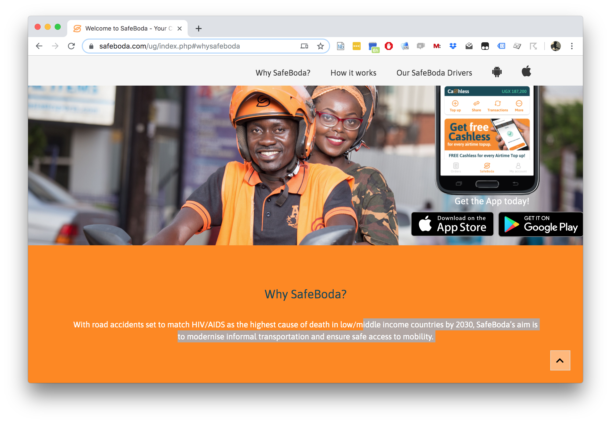
SafeBoda

With road accidents set to match HIV/AIDS as the highest cause of death in low/middle income countries by 2030, SafeBoda’s aim is to modernise informal transportation and ensure safe access to mobility.

Ride Allocation Prediction

Ride Sharing: Service Oriented

Ride Sharing: Data Oriented

Ride Sharing: Hypothetical

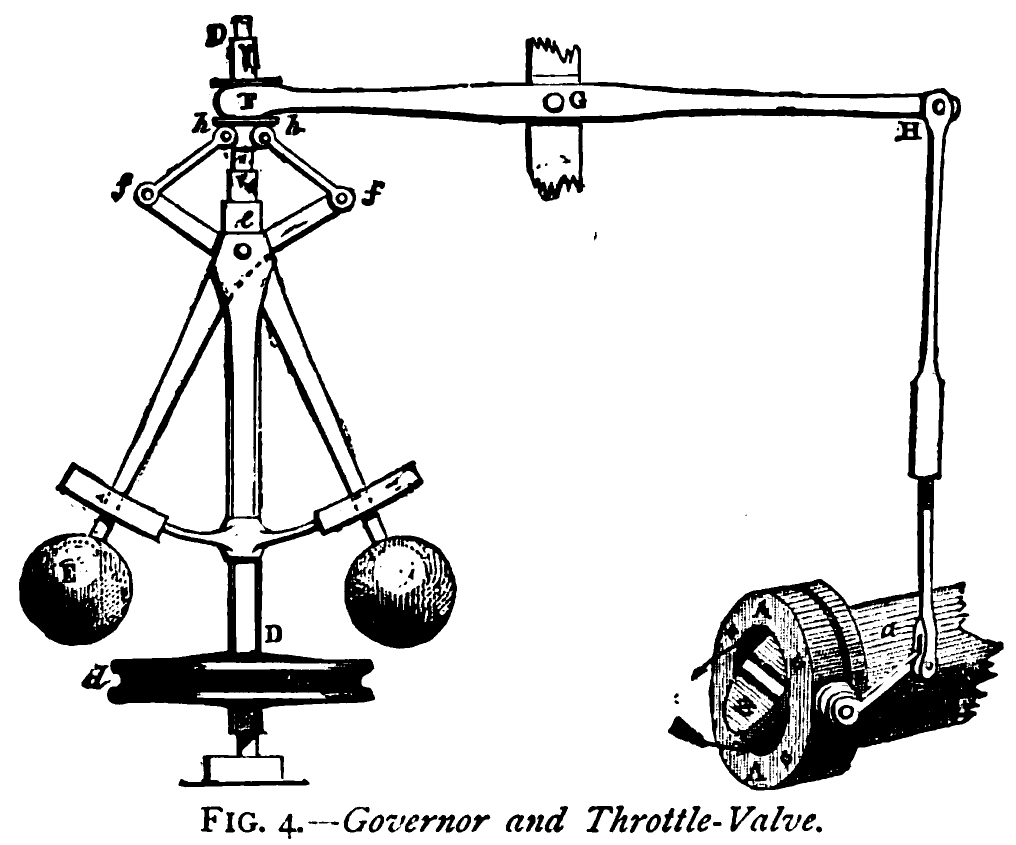
Information Dynamics

• Potential for information feedback loops.
• Hypothetical streams are instantiated.
• Nature hypothesis (e.g. price prediction) can effect reality.
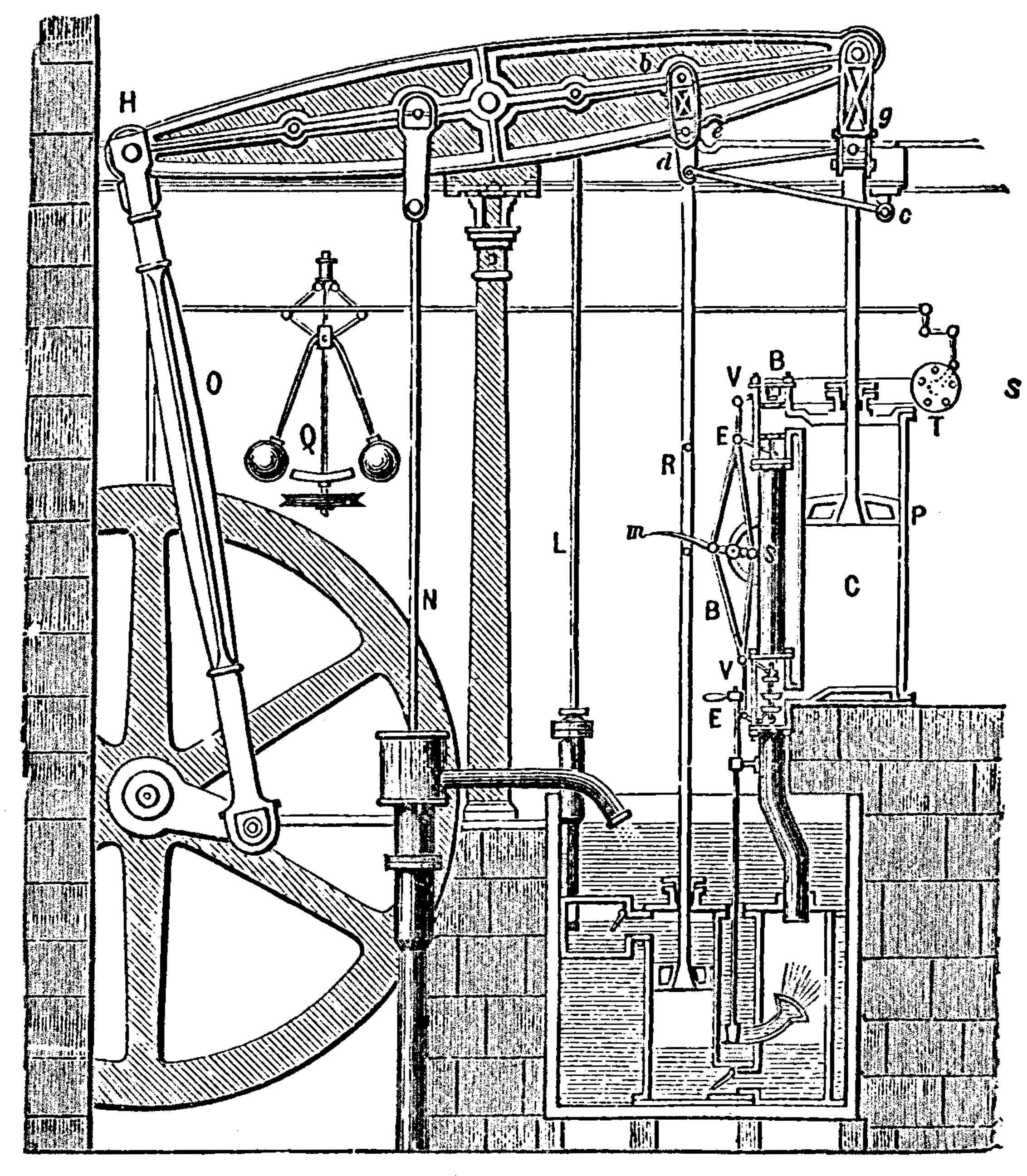
• Leads to information dynamics, similar to dynamics of governors.
• See e.g. Closed Loop Data Science at Glasgow.

Xfer

Work by Andreas Damianou, Pablo Moreno, Keerthana Elango, Jordan Massiah, Cliff McCollum Available on Github

Xfer

• Deep learning transfer tutorial.

Emukit

Emukit

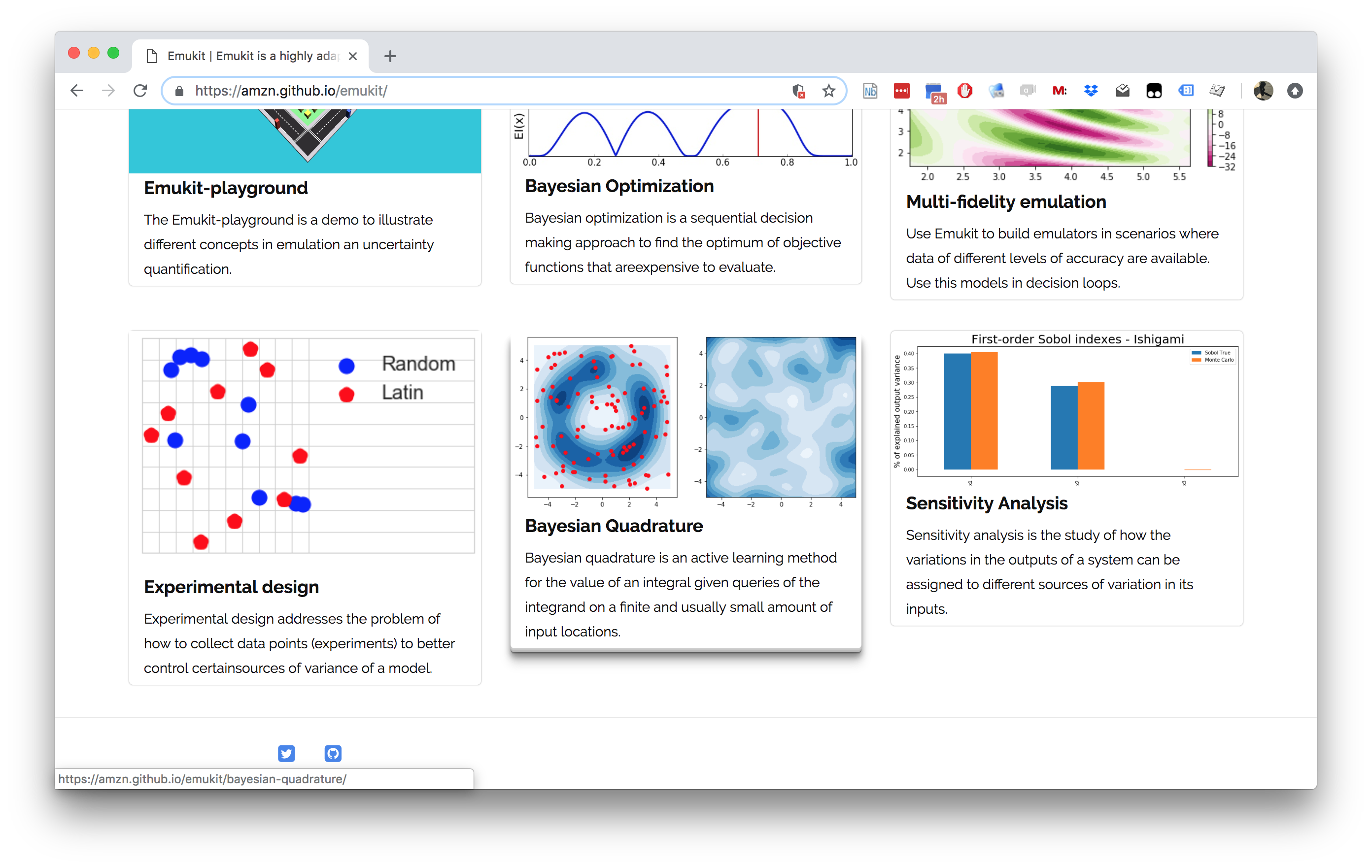
Emukit

• Work by Javier Gonzalez, Andrei Paleyes, Mark Pullin, Maren Mahsereci, Alex Gessner, Aaron Klein.
• Available on Github
• Example sensitivity notebook.

Emukit Software

• Multi-fidelity emulation: build surrogate models for multiple sources of information;
• Bayesian optimisation: optimise physical experiments and tune parameters ML algorithms;
• Experimental design/Active learning: design experiments and perform active learning with ML models;
• Sensitivity analysis: analyse the influence of inputs on the outputs
• Bayesian quadrature: compute integrals of functions that are expensive to evaluate.

–> ### Outlook for Machine Learning

• Risen to prominence to scale our activities.
• To scale activities need more computer based automation.
• Machine learning allows us to automate processes previously out of reach.

Conclusion

• Technologically evolving environment.
• ML is a key component of decision making.
• Data is the key component of ML.
• ML is critically dependent on data.
• Challenges in problem Decomposition, Data curation and model Deployment

Thanks!

• twitter: @lawrennd
• podcast: The Talking Machines

• Guardian article on The data-driven economy will help marketers exploit us

• Guardian article on How African can benefit from the data revolution

• Guardian article on Data Trusts

• Guardian article on Digital Oligarchies

• Guardian article on Information Feudalism

• Blog post on Lies, Damned Lies and Big Data

• Blog post on System Zero

• Andrej Karpathy’s Medium Post

• Blog post on Data Readiness Levels

• Blog post on Three Data Science Challenges

• Blog post on The 3Ds of Machine Learning Systems Design

• Blog post on Data Science as Debugging

References

Andrade-Pacheco, R., Mubangizi, M., Quinn, J., Lawrence, N.D., 2014. Consistent mapping of government malaria records across a changing territory delimitation. Malaria Journal 13. https://doi.org/10.1186/1475-2875-13-S1-P5
Delacroix, S., Lawrence, N.D., 2019. Bottom-up data trusts: Disturbing the “one size fits all” approach to data governance. International Data Privacy Law. https://doi.org/10.1093/idpl/ipz014
Edwards, L., 2004. The problem with privacy. International Review of Law Computers & Technology 18, 263–294.
Lawrence, N.D., 2017a. Living together: Mind and machine intelligence. arXiv.
Lawrence, N.D., 2017b. Data readiness levels. arXiv.
Lawrence, N.D., 2016. Data trusts could allay our privacy fears.
Lawrence, N.D., 2015a. Beware the rise of the digital oligarchy.
Lawrence, N.D., 2015b. The information barons threaten our autonomy and our privacy.
Mubangizi, M., Andrade-Pacheco, R., Smith, M.T., Quinn, J., Lawrence, N.D., 2014. Malaria surveillance with multiple data sources using Gaussian process models, in: 1st International Conference on the Use of Mobile ICT in Africa.
Russakovsky, O., Deng, J., Su, H., Krause, J., Satheesh, S., Ma, S., Huang, Z., Karpathy, A., Khosla, A., Bernstein, M., Berg, A.C., Fei-Fei, L., 2015. ImageNet Large Scale Visual Recognition Challenge. International Journal of Computer Vision (IJCV) 115, 211–252. https://doi.org/10.1007/s11263-015-0816-y
Taigman, Y., Yang, M., Ranzato, M., Wolf, L., 2014. DeepFace: Closing the gap to human-level performance in face verification, in: Proceedings of the IEEE Computer Society Conference on Computer Vision and Pattern Recognition. https://doi.org/10.1109/CVPR.2014.220