\[\newcommand{\tk}[1]{} %\newcommand{\tk}[1]{\textbf{TK}: #1} \newcommand{\Amatrix}{\mathbf{A}} \newcommand{\KL}[2]{\text{KL}\left( #1\,\|\,#2 \right)} \newcommand{\Kaast}{\kernelMatrix_{\mathbf{ \ast}\mathbf{ \ast}}} \newcommand{\Kastu}{\kernelMatrix_{\mathbf{ \ast} \inducingVector}} \newcommand{\Kff}{\kernelMatrix_{\mappingFunctionVector \mappingFunctionVector}} \newcommand{\Kfu}{\kernelMatrix_{\mappingFunctionVector \inducingVector}} \newcommand{\Kuast}{\kernelMatrix_{\inducingVector \bf\ast}} \newcommand{\Kuf}{\kernelMatrix_{\inducingVector \mappingFunctionVector}} \newcommand{\Kuu}{\kernelMatrix_{\inducingVector \inducingVector}} \newcommand{\Kuui}{\Kuu^{-1}} \newcommand{\Qaast}{\mathbf{Q}_{\bf \ast \ast}} \newcommand{\Qastf}{\mathbf{Q}_{\ast \mappingFunction}} \newcommand{\Qfast}{\mathbf{Q}_{\mappingFunctionVector \bf \ast}} \newcommand{\Qff}{\mathbf{Q}_{\mappingFunctionVector \mappingFunctionVector}} \newcommand{\aMatrix}{\mathbf{A}} \newcommand{\aScalar}{a} \newcommand{\aVector}{\mathbf{a}} \newcommand{\acceleration}{a} \newcommand{\bMatrix}{\mathbf{B}} \newcommand{\bScalar}{b} \newcommand{\bVector}{\mathbf{b}} \newcommand{\basisFunc}{\phi} \newcommand{\basisFuncVector}{\boldsymbol{ \basisFunc}} \newcommand{\basisFunction}{\phi} \newcommand{\basisLocation}{\mu} \newcommand{\basisMatrix}{\boldsymbol{ \Phi}} \newcommand{\basisScalar}{\basisFunction} \newcommand{\basisVector}{\boldsymbol{ \basisFunction}} \newcommand{\activationFunction}{\phi} \newcommand{\activationMatrix}{\boldsymbol{ \Phi}} \newcommand{\activationScalar}{\basisFunction} \newcommand{\activationVector}{\boldsymbol{ \basisFunction}} \newcommand{\bigO}{\mathcal{O}} \newcommand{\binomProb}{\pi} \newcommand{\cMatrix}{\mathbf{C}} \newcommand{\cbasisMatrix}{\hat{\boldsymbol{ \Phi}}} \newcommand{\cdataMatrix}{\hat{\dataMatrix}} \newcommand{\cdataScalar}{\hat{\dataScalar}} \newcommand{\cdataVector}{\hat{\dataVector}} \newcommand{\centeredKernelMatrix}{\mathbf{ \MakeUppercase{\centeredKernelScalar}}} \newcommand{\centeredKernelScalar}{b} \newcommand{\centeredKernelVector}{\centeredKernelScalar} \newcommand{\centeringMatrix}{\mathbf{H}} \newcommand{\chiSquaredDist}[2]{\chi_{#1}^{2}\left(#2\right)} \newcommand{\chiSquaredSamp}[1]{\chi_{#1}^{2}} \newcommand{\conditionalCovariance}{\boldsymbol{ \Sigma}} \newcommand{\coregionalizationMatrix}{\mathbf{B}} \newcommand{\coregionalizationScalar}{b} \newcommand{\coregionalizationVector}{\mathbf{ \coregionalizationScalar}} \newcommand{\covDist}[2]{\text{cov}_{#2}\left(#1\right)} \newcommand{\covSamp}[1]{\text{cov}\left(#1\right)} \newcommand{\covarianceScalar}{c} \newcommand{\covarianceVector}{\mathbf{ \covarianceScalar}} \newcommand{\covarianceMatrix}{\mathbf{C}} \newcommand{\covarianceMatrixTwo}{\boldsymbol{ \Sigma}} \newcommand{\croupierScalar}{s} \newcommand{\croupierVector}{\mathbf{ \croupierScalar}} \newcommand{\croupierMatrix}{\mathbf{ \MakeUppercase{\croupierScalar}}} \newcommand{\dataDim}{p} \newcommand{\dataIndex}{i} \newcommand{\dataIndexTwo}{j} \newcommand{\dataMatrix}{\mathbf{Y}} \newcommand{\dataScalar}{y} \newcommand{\dataSet}{\mathcal{D}} \newcommand{\dataStd}{\sigma} \newcommand{\dataVector}{\mathbf{ \dataScalar}} \newcommand{\decayRate}{d} \newcommand{\degreeMatrix}{\mathbf{ \MakeUppercase{\degreeScalar}}} \newcommand{\degreeScalar}{d} \newcommand{\degreeVector}{\mathbf{ \degreeScalar}} % Already defined by latex %\newcommand{\det}[1]{\left|#1\right|} \newcommand{\diag}[1]{\text{diag}\left(#1\right)} \newcommand{\diagonalMatrix}{\mathbf{D}} \newcommand{\diff}[2]{\frac{\text{d}#1}{\text{d}#2}} \newcommand{\diffTwo}[2]{\frac{\text{d}^2#1}{\text{d}#2^2}} \newcommand{\displacement}{x} \newcommand{\displacementVector}{\textbf{\displacement}} \newcommand{\distanceMatrix}{\mathbf{ \MakeUppercase{\distanceScalar}}} \newcommand{\distanceScalar}{d} \newcommand{\distanceVector}{\mathbf{ \distanceScalar}} \newcommand{\eigenvaltwo}{\ell} \newcommand{\eigenvaltwoMatrix}{\mathbf{L}} \newcommand{\eigenvaltwoVector}{\mathbf{l}} \newcommand{\eigenvalue}{\lambda} \newcommand{\eigenvalueMatrix}{\boldsymbol{ \Lambda}} \newcommand{\eigenvalueVector}{\boldsymbol{ \lambda}} \newcommand{\eigenvector}{\mathbf{ \eigenvectorScalar}} \newcommand{\eigenvectorMatrix}{\mathbf{U}} \newcommand{\eigenvectorScalar}{u} \newcommand{\eigenvectwo}{\mathbf{v}} \newcommand{\eigenvectwoMatrix}{\mathbf{V}} \newcommand{\eigenvectwoScalar}{v} \newcommand{\entropy}[1]{\mathcal{H}\left(#1\right)} \newcommand{\errorFunction}{E} \newcommand{\expDist}[2]{\left<#1\right>_{#2}} \newcommand{\expSamp}[1]{\left<#1\right>} \newcommand{\expectation}[1]{\left\langle #1 \right\rangle } \newcommand{\expectationDist}[2]{\left\langle #1 \right\rangle _{#2}} \newcommand{\expectedDistanceMatrix}{\mathcal{D}} \newcommand{\eye}{\mathbf{I}} \newcommand{\fantasyDim}{r} \newcommand{\fantasyMatrix}{\mathbf{ \MakeUppercase{\fantasyScalar}}} \newcommand{\fantasyScalar}{z} \newcommand{\fantasyVector}{\mathbf{ \fantasyScalar}} \newcommand{\featureStd}{\varsigma} \newcommand{\gammaCdf}[3]{\mathcal{GAMMA CDF}\left(#1|#2,#3\right)} \newcommand{\gammaDist}[3]{\mathcal{G}\left(#1|#2,#3\right)} \newcommand{\gammaSamp}[2]{\mathcal{G}\left(#1,#2\right)} \newcommand{\gaussianDist}[3]{\mathcal{N}\left(#1|#2,#3\right)} \newcommand{\gaussianSamp}[2]{\mathcal{N}\left(#1,#2\right)} \newcommand{\given}{|} \newcommand{\half}{\frac{1}{2}} \newcommand{\heaviside}{H} \newcommand{\hiddenMatrix}{\mathbf{ \MakeUppercase{\hiddenScalar}}} \newcommand{\hiddenScalar}{h} \newcommand{\hiddenVector}{\mathbf{ \hiddenScalar}} \newcommand{\identityMatrix}{\eye} \newcommand{\inducingInputScalar}{z} \newcommand{\inducingInputVector}{\mathbf{ \inducingInputScalar}} \newcommand{\inducingInputMatrix}{\mathbf{Z}} \newcommand{\inducingScalar}{u} \newcommand{\inducingVector}{\mathbf{ \inducingScalar}} \newcommand{\inducingMatrix}{\mathbf{U}} \newcommand{\inlineDiff}[2]{\text{d}#1/\text{d}#2} \newcommand{\inputDim}{q} \newcommand{\inputMatrix}{\mathbf{X}} \newcommand{\inputScalar}{x} \newcommand{\inputSpace}{\mathcal{X}} \newcommand{\inputVals}{\inputVector} \newcommand{\inputVector}{\mathbf{ \inputScalar}} \newcommand{\iterNum}{k} \newcommand{\kernel}{\kernelScalar} \newcommand{\kernelMatrix}{\mathbf{K}} \newcommand{\kernelScalar}{k} \newcommand{\kernelVector}{\mathbf{ \kernelScalar}} \newcommand{\kff}{\kernelScalar_{\mappingFunction \mappingFunction}} \newcommand{\kfu}{\kernelVector_{\mappingFunction \inducingScalar}} \newcommand{\kuf}{\kernelVector_{\inducingScalar \mappingFunction}} \newcommand{\kuu}{\kernelVector_{\inducingScalar \inducingScalar}} \newcommand{\lagrangeMultiplier}{\lambda} \newcommand{\lagrangeMultiplierMatrix}{\boldsymbol{ \Lambda}} \newcommand{\lagrangian}{L} \newcommand{\laplacianFactor}{\mathbf{ \MakeUppercase{\laplacianFactorScalar}}} \newcommand{\laplacianFactorScalar}{m} \newcommand{\laplacianFactorVector}{\mathbf{ \laplacianFactorScalar}} \newcommand{\laplacianMatrix}{\mathbf{L}} \newcommand{\laplacianScalar}{\ell} \newcommand{\laplacianVector}{\mathbf{ \ell}} \newcommand{\latentDim}{q} \newcommand{\latentDistanceMatrix}{\boldsymbol{ \Delta}} \newcommand{\latentDistanceScalar}{\delta} \newcommand{\latentDistanceVector}{\boldsymbol{ \delta}} \newcommand{\latentForce}{f} \newcommand{\latentFunction}{u} \newcommand{\latentFunctionVector}{\mathbf{ \latentFunction}} \newcommand{\latentFunctionMatrix}{\mathbf{ \MakeUppercase{\latentFunction}}} \newcommand{\latentIndex}{j} \newcommand{\latentScalar}{z} \newcommand{\latentVector}{\mathbf{ \latentScalar}} \newcommand{\latentMatrix}{\mathbf{Z}} \newcommand{\learnRate}{\eta} \newcommand{\lengthScale}{\ell} \newcommand{\rbfWidth}{\ell} \newcommand{\likelihoodBound}{\mathcal{L}} \newcommand{\likelihoodFunction}{L} \newcommand{\locationScalar}{\mu} \newcommand{\locationVector}{\boldsymbol{ \locationScalar}} \newcommand{\locationMatrix}{\mathbf{M}} \newcommand{\variance}[1]{\text{var}\left( #1 \right)} \newcommand{\mappingFunction}{f} \newcommand{\mappingFunctionMatrix}{\mathbf{F}} \newcommand{\mappingFunctionTwo}{g} \newcommand{\mappingFunctionTwoMatrix}{\mathbf{G}} \newcommand{\mappingFunctionTwoVector}{\mathbf{ \mappingFunctionTwo}} \newcommand{\mappingFunctionVector}{\mathbf{ \mappingFunction}} \newcommand{\scaleScalar}{s} \newcommand{\mappingScalar}{w} \newcommand{\mappingVector}{\mathbf{ \mappingScalar}} \newcommand{\mappingMatrix}{\mathbf{W}} \newcommand{\mappingScalarTwo}{v} \newcommand{\mappingVectorTwo}{\mathbf{ \mappingScalarTwo}} \newcommand{\mappingMatrixTwo}{\mathbf{V}} \newcommand{\maxIters}{K} \newcommand{\meanMatrix}{\mathbf{M}} \newcommand{\meanScalar}{\mu} \newcommand{\meanTwoMatrix}{\mathbf{M}} \newcommand{\meanTwoScalar}{m} \newcommand{\meanTwoVector}{\mathbf{ \meanTwoScalar}} \newcommand{\meanVector}{\boldsymbol{ \meanScalar}} \newcommand{\mrnaConcentration}{m} \newcommand{\naturalFrequency}{\omega} \newcommand{\neighborhood}[1]{\mathcal{N}\left( #1 \right)} \newcommand{\neilurl}{http://inverseprobability.com/} \newcommand{\noiseMatrix}{\boldsymbol{ E}} \newcommand{\noiseScalar}{\epsilon} \newcommand{\noiseVector}{\boldsymbol{ \epsilon}} \newcommand{\norm}[1]{\left\Vert #1 \right\Vert} \newcommand{\normalizedLaplacianMatrix}{\hat{\mathbf{L}}} \newcommand{\normalizedLaplacianScalar}{\hat{\ell}} \newcommand{\normalizedLaplacianVector}{\hat{\mathbf{ \ell}}} \newcommand{\numActive}{m} \newcommand{\numBasisFunc}{m} \newcommand{\numComponents}{m} \newcommand{\numComps}{K} \newcommand{\numData}{n} \newcommand{\numFeatures}{K} \newcommand{\numHidden}{h} \newcommand{\numInducing}{m} \newcommand{\numLayers}{\ell} \newcommand{\numNeighbors}{K} \newcommand{\numSequences}{s} \newcommand{\numSuccess}{s} \newcommand{\numTasks}{m} \newcommand{\numTime}{T} \newcommand{\numTrials}{S} \newcommand{\outputIndex}{j} \newcommand{\paramVector}{\boldsymbol{ \theta}} \newcommand{\parameterMatrix}{\boldsymbol{ \Theta}} \newcommand{\parameterScalar}{\theta} \newcommand{\parameterVector}{\boldsymbol{ \parameterScalar}} \newcommand{\partDiff}[2]{\frac{\partial#1}{\partial#2}} \newcommand{\precisionScalar}{j} \newcommand{\precisionVector}{\mathbf{ \precisionScalar}} \newcommand{\precisionMatrix}{\mathbf{J}} \newcommand{\pseudotargetScalar}{\widetilde{y}} \newcommand{\pseudotargetVector}{\mathbf{ \pseudotargetScalar}} \newcommand{\pseudotargetMatrix}{\mathbf{ \widetilde{Y}}} \newcommand{\rank}[1]{\text{rank}\left(#1\right)} \newcommand{\rayleighDist}[2]{\mathcal{R}\left(#1|#2\right)} \newcommand{\rayleighSamp}[1]{\mathcal{R}\left(#1\right)} \newcommand{\responsibility}{r} \newcommand{\rotationScalar}{r} \newcommand{\rotationVector}{\mathbf{ \rotationScalar}} \newcommand{\rotationMatrix}{\mathbf{R}} \newcommand{\sampleCovScalar}{s} \newcommand{\sampleCovVector}{\mathbf{ \sampleCovScalar}} \newcommand{\sampleCovMatrix}{\mathbf{s}} \newcommand{\scalarProduct}[2]{\left\langle{#1},{#2}\right\rangle} \newcommand{\sign}[1]{\text{sign}\left(#1\right)} \newcommand{\sigmoid}[1]{\sigma\left(#1\right)} \newcommand{\singularvalue}{\ell} \newcommand{\singularvalueMatrix}{\mathbf{L}} \newcommand{\singularvalueVector}{\mathbf{l}} \newcommand{\sorth}{\mathbf{u}} \newcommand{\spar}{\lambda} \newcommand{\trace}[1]{\text{tr}\left(#1\right)} \newcommand{\BasalRate}{B} \newcommand{\DampingCoefficient}{C} \newcommand{\DecayRate}{D} \newcommand{\Displacement}{X} \newcommand{\LatentForce}{F} \newcommand{\Mass}{M} \newcommand{\Sensitivity}{S} \newcommand{\basalRate}{b} \newcommand{\dampingCoefficient}{c} \newcommand{\mass}{m} \newcommand{\sensitivity}{s} \newcommand{\springScalar}{\kappa} \newcommand{\springVector}{\boldsymbol{ \kappa}} \newcommand{\springMatrix}{\boldsymbol{ \mathcal{K}}} \newcommand{\tfConcentration}{p} \newcommand{\tfDecayRate}{\delta} \newcommand{\tfMrnaConcentration}{f} \newcommand{\tfVector}{\mathbf{ \tfConcentration}} \newcommand{\velocity}{v} \newcommand{\sufficientStatsScalar}{g} \newcommand{\sufficientStatsVector}{\mathbf{ \sufficientStatsScalar}} \newcommand{\sufficientStatsMatrix}{\mathbf{G}} \newcommand{\switchScalar}{s} \newcommand{\switchVector}{\mathbf{ \switchScalar}} \newcommand{\switchMatrix}{\mathbf{S}} \newcommand{\tr}[1]{\text{tr}\left(#1\right)} \newcommand{\loneNorm}[1]{\left\Vert #1 \right\Vert_1} \newcommand{\ltwoNorm}[1]{\left\Vert #1 \right\Vert_2} \newcommand{\onenorm}[1]{\left\vert#1\right\vert_1} \newcommand{\twonorm}[1]{\left\Vert #1 \right\Vert} \newcommand{\vScalar}{v} \newcommand{\vVector}{\mathbf{v}} \newcommand{\vMatrix}{\mathbf{V}} \newcommand{\varianceDist}[2]{\text{var}_{#2}\left( #1 \right)} % Already defined by latex %\newcommand{\vec}{#1:} \newcommand{\vecb}[1]{\left(#1\right):} \newcommand{\weightScalar}{w} \newcommand{\weightVector}{\mathbf{ \weightScalar}} \newcommand{\weightMatrix}{\mathbf{W}} \newcommand{\weightedAdjacencyMatrix}{\mathbf{A}} \newcommand{\weightedAdjacencyScalar}{a} \newcommand{\weightedAdjacencyVector}{\mathbf{ \weightedAdjacencyScalar}} \newcommand{\onesVector}{\mathbf{1}} \newcommand{\zerosVector}{\mathbf{0}} \]

Towards Machine Learning Systems Design

Neil D. Lawrence

Department of Computing Science, University of Glasgow

What is Machine Learning?

\[ \text{data} + \text{model} \xrightarrow{\text{compute}} \text{prediction}\]

  • data : observations, could be actively or passively acquired (meta-data).
  • model : assumptions, based on previous experience (other data! transfer learning etc), or beliefs about the regularities of the universe. Inductive bias.
  • prediction : an action to be taken or a categorization or a quality score.

What is Machine Learning?

\[\text{data} + \text{model} \xrightarrow{\text{compute}} \text{prediction}\]

  • To combine data with a model need:
  • a prediction function \(\mappingFunction (\cdot)\) includes our beliefs about the regularities of the universe
  • an objective function \(\errorFunction (\cdot)\) defines the cost of misprediction.

Machine Learning

  • Driver of two different domains:
    1. Data Science: arises from the fact that we now capture data by happenstance.
    2. Artificial Intelligence: emulation of human behaviour.
  • Connection: Internet of Things

Machine Learning

  • Driver of two different domains:
    1. Data Science: arises from the fact that we now capture data by happenstance.
    2. Artificial Intelligence: emulation of human behaviour.
  • Connection: Internet of Things

Machine Learning

  • Driver of two different domains:
    1. Data Science: arises from the fact that we now capture data by happenstance.
    2. Artificial Intelligence: emulation of human behaviour.
  • Connection: Internet of People

Convention for the Protection of Individuals with regard to Automatic Processing of Personal Data (1981/1/28)

What does Machine Learning do?

  • ML Automates through Data
    • Strongly related to statistics.
    • Field underpins revolution in data science and AI
  • With AI:
    • logic, robotics, computer vision, speech
  • With Data Science:
    • databases, data mining, statistics, visualization

Embodiment Factors
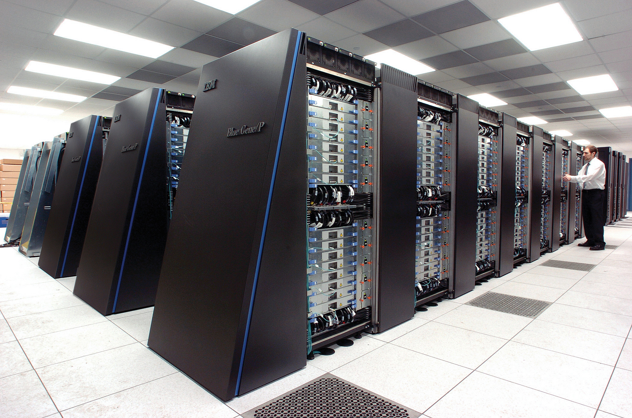
compute \[\approx 100 \text{ gigaflops}\] \[\approx 16 \text{ petaflops}\]
communicate \[1 \text{ gigbit/s}\] \[100 \text{ bit/s}\]
(compute/communicate) \[10^{4}\] \[10^{14}\]

See “Living Together: Mind and Machine Intelligence” Lawrence (2017)

.

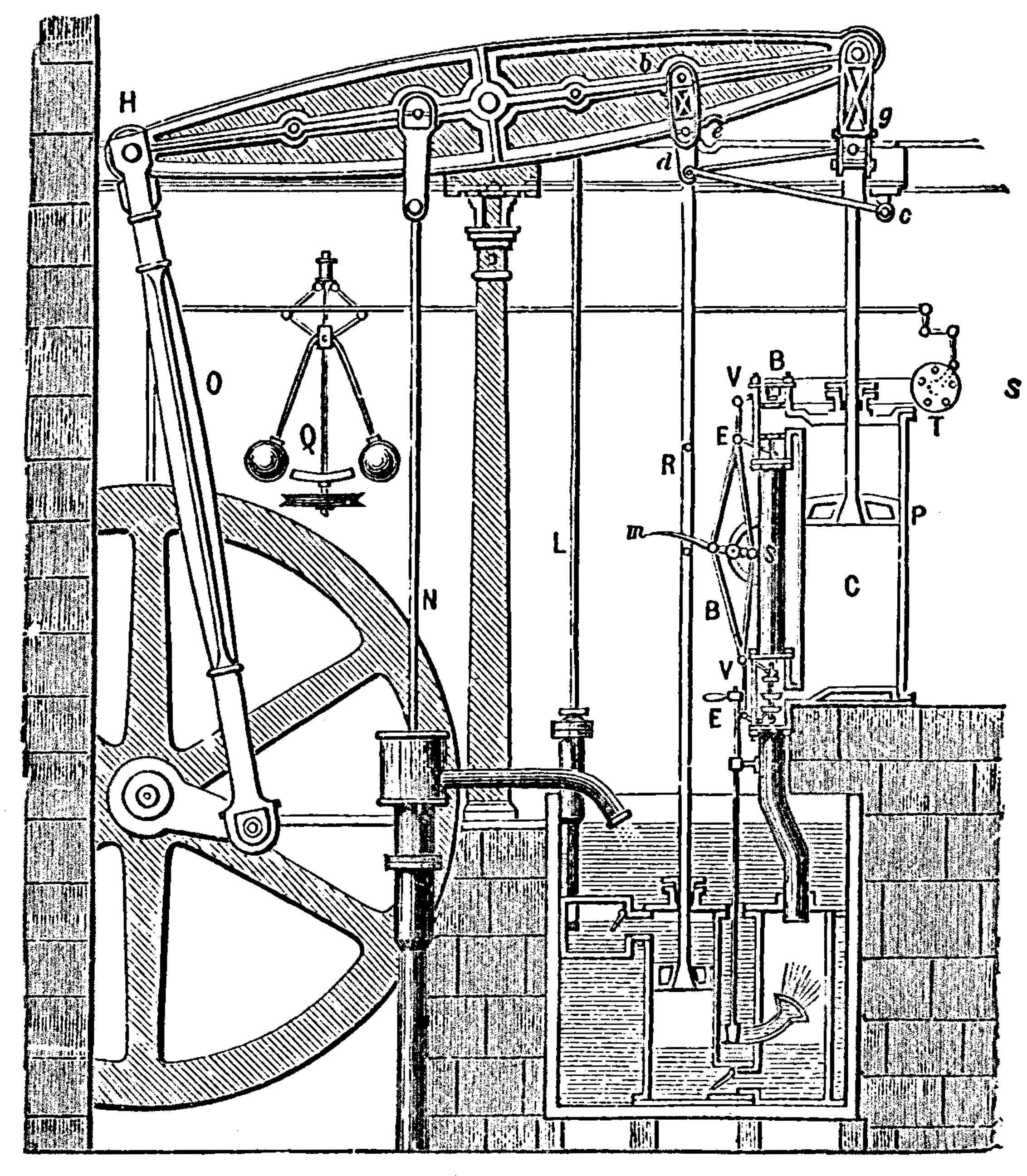
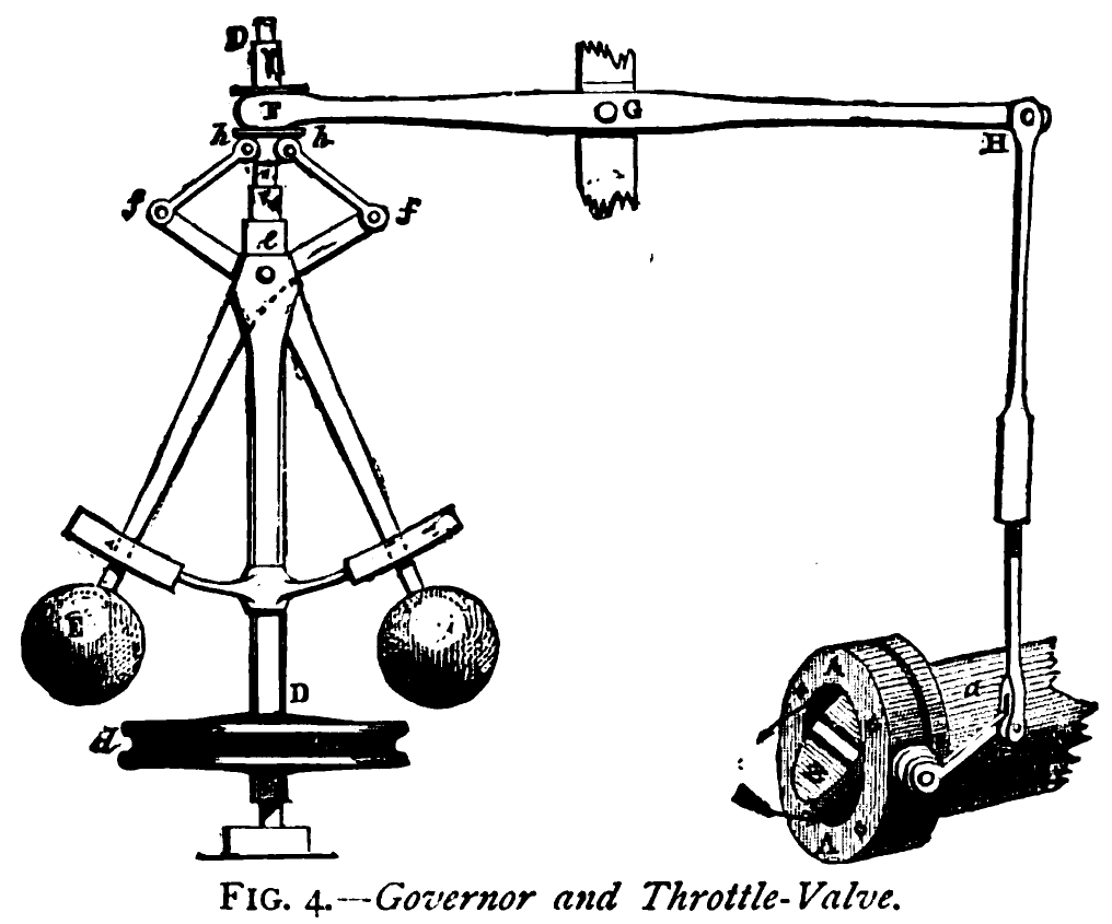
Evolved Relationship

Evolved Relationship

What does Machine Learning do?

  • Automation scales by codifying processes and automating them.
  • Need:
    • Interconnected components
    • Compatible components
  • Early examples:
    • cf Colt 45, Ford Model T

Codify Through Mathematical Functions

  • How does machine learning work?
  • Jumper (jersey/sweater) purchase with logistic regression

\[ \text{odds} = \frac{p(\text{bought})}{p(\text{not bought})} \]

\[ \log \text{odds} = \beta_0 + \beta_1 \text{age} + \beta_2 \text{latitude}.\]

Codify Through Mathematical Functions

  • How does machine learning work?
  • Jumper (jersey/sweater) purchase with logistic regression

\[ p(\text{bought}) = \sigmoid{\beta_0 + \beta_1 \text{age} + \beta_2 \text{latitude}}.\]

Codify Through Mathematical Functions

  • How does machine learning work?
  • Jumper (jersey/sweater) purchase with logistic regression

\[ p(\text{bought}) = \sigmoid{\boldsymbol{\beta}^\top \inputVector}.\]

Codify Through Mathematical Functions

  • How does machine learning work?
  • Jumper (jersey/sweater) purchase with logistic regression

\[ \dataScalar = \mappingFunction\left(\inputVector, \boldsymbol{\beta}\right).\]

We call \(\mappingFunction(\cdot)\) the prediction function.

Fit to Data

  • Use an objective function

\[\errorFunction(\boldsymbol{\beta}, \dataMatrix, \inputMatrix)\]

  • E.g. least squares \[\errorFunction(\boldsymbol{\beta}, \dataMatrix, \inputMatrix) = \sum_{i=1}^\numData \left(\dataScalar_i - \mappingFunction(\inputVector_i, \boldsymbol{\beta})\right)^2.\]

Two Components

  • Prediction function, \(\mappingFunction(\cdot)\)
  • Objective function, \(\errorFunction(\cdot)\)

Deep Learning

  • These are interpretable models: vital for disease modeling etc.

  • Modern machine learning methods are less interpretable

  • Example: face recognition

DeepFace

Outline of the DeepFace architecture. A front-end of a single convolution-pooling-convolution filtering on the rectified input, followed by three locally-connected layers and two fully-connected layers. Color illustrates feature maps produced at each layer. The net includes more than 120 million parameters, where more than 95% come from the local and fully connected.

Source: DeepFace (Taigman et al., 2014)

Deep Learning as Pinball

Olympic Marathon Data

  • Gold medal times for Olympic Marathon since 1896.
  • Marathons before 1924 didn’t have a standardised distance.
  • Present results using pace per km.
  • In 1904 Marathon was badly organised leading to very slow times.
Image from Wikimedia Commons http://bit.ly/16kMKHQ

Olympic Marathon Data

Alan Turing

Probability Winning Olympics?

  • He was a formidable Marathon runner.
  • In 1946 he ran a time 2 hours 46 minutes.
    • That’s a pace of 3.95 min/km.
  • What is the probability he would have won an Olympics if one had been held in 1946?

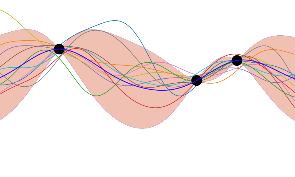
Olympic Marathon Data GP

Deep GP Fit

  • Can a Deep Gaussian process help?

  • Deep GP is one GP feeding into another.

Olympic Marathon Data Deep GP

Olympic Marathon Data Deep GP

Olympic Marathon Data Latent 1

Olympic Marathon Data Latent 2

Olympic Marathon Pinball Plot

Supply Chain

Cromford

Deep Freeze

Deep Freeze
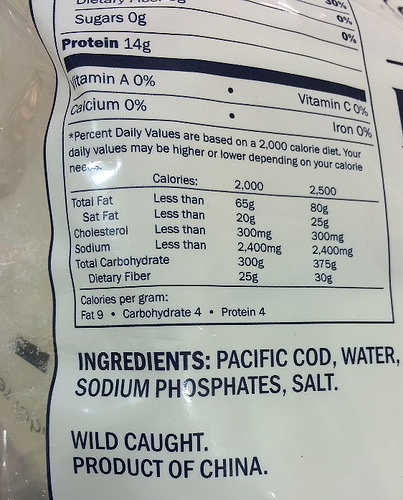
Machine Learning in Supply Chain

  • Supply chain: Large Automated Decision Making Network
  • Major Challenge:
    • We have a mechanistic understanding of supply chain.
    • Machine learning is a data driven technology.

Deploying Artificial Intelligence

  • Challenges in deploying AI.
  • Currently this is in the form of “machine learning systems”

Internet of People

  • Fog computing: barrier between cloud and device blurring.
    • Computing on the Edge
  • Complex feedback between algorithm and implementation

Deploying ML in Real World: Machine Learning Systems Design

  • Major new challenge for systems designers.
  • Internet of Intelligence but currently:
    • AI systems are fragile

Machine Learning Systems Design

Fragility of AI Systems

  • They are componentwise built from ML Capabilities.
  • Each capability is independently constructed and verified.
    • Pedestrian detection
    • Road line detection
  • Important for verification purposes.

Pigeonholing

Robust

  • Need to move beyond pigeonholing tasks.
  • Need new approaches to both the design of the individual components, and the combination of components within our AI systems.

Rapid Reimplementation

  • Whole systems are being deployed.
  • But they change their environment.
  • The experience evolved adversarial behaviour.

Machine Learning Systems Design

Adversaries

  • Stuxnet
  • Mischevious-Adversarial

An Intelligent System

Joint work with M. Milo

An Intelligent System

Joint work with M. Milo

Peppercorns

  • A new name for system failures which aren’t bugs.
  • Difference between finding a fly in your soup vs a peppercorn in your soup.

Peppercorns

Turnaround And Update

  • There is a massive need for turn around and update
  • A redeploy of the entire system.
    • This involves changing the way we design and deploy.
  • Interface between security engineering and machine learning.

Emukit
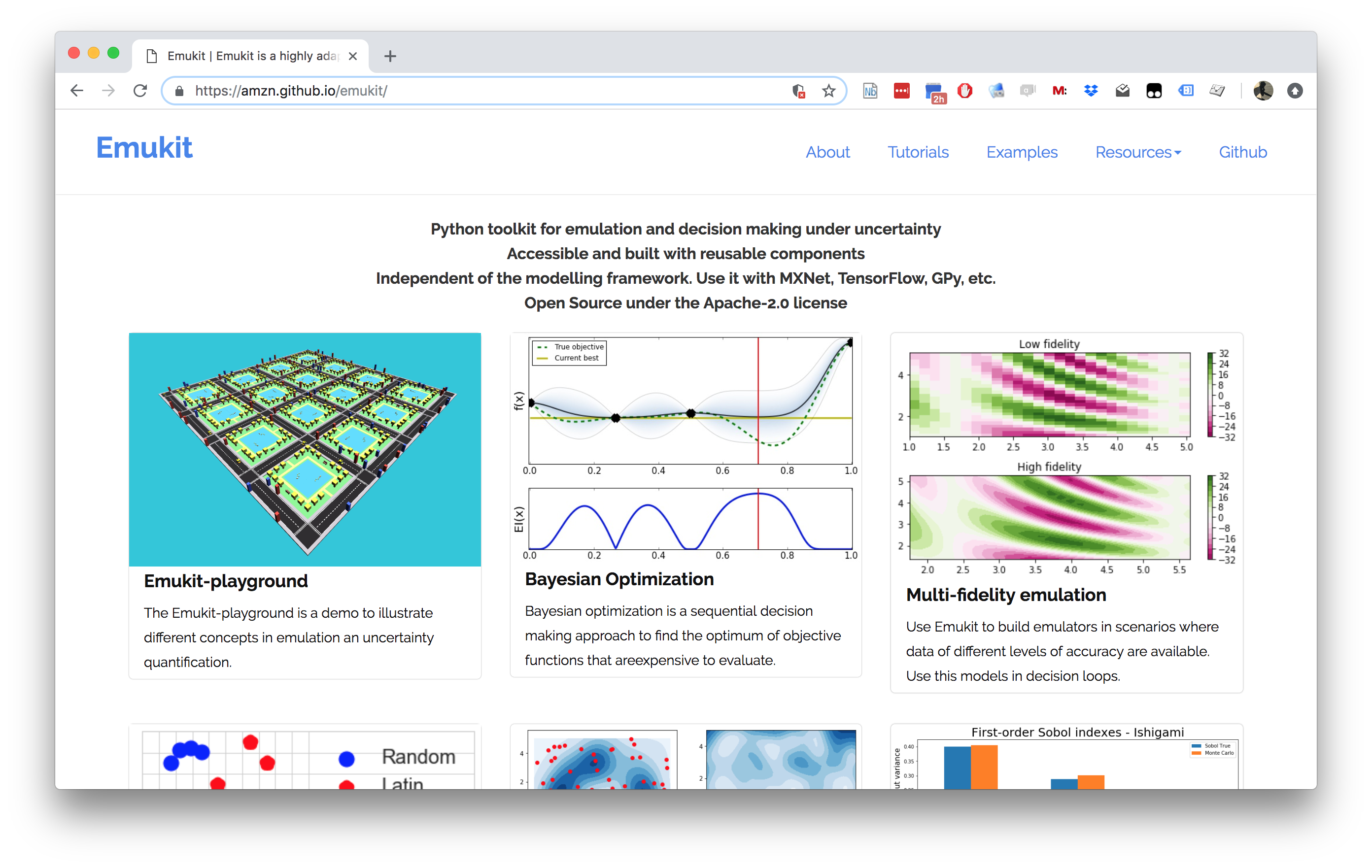
Emukit
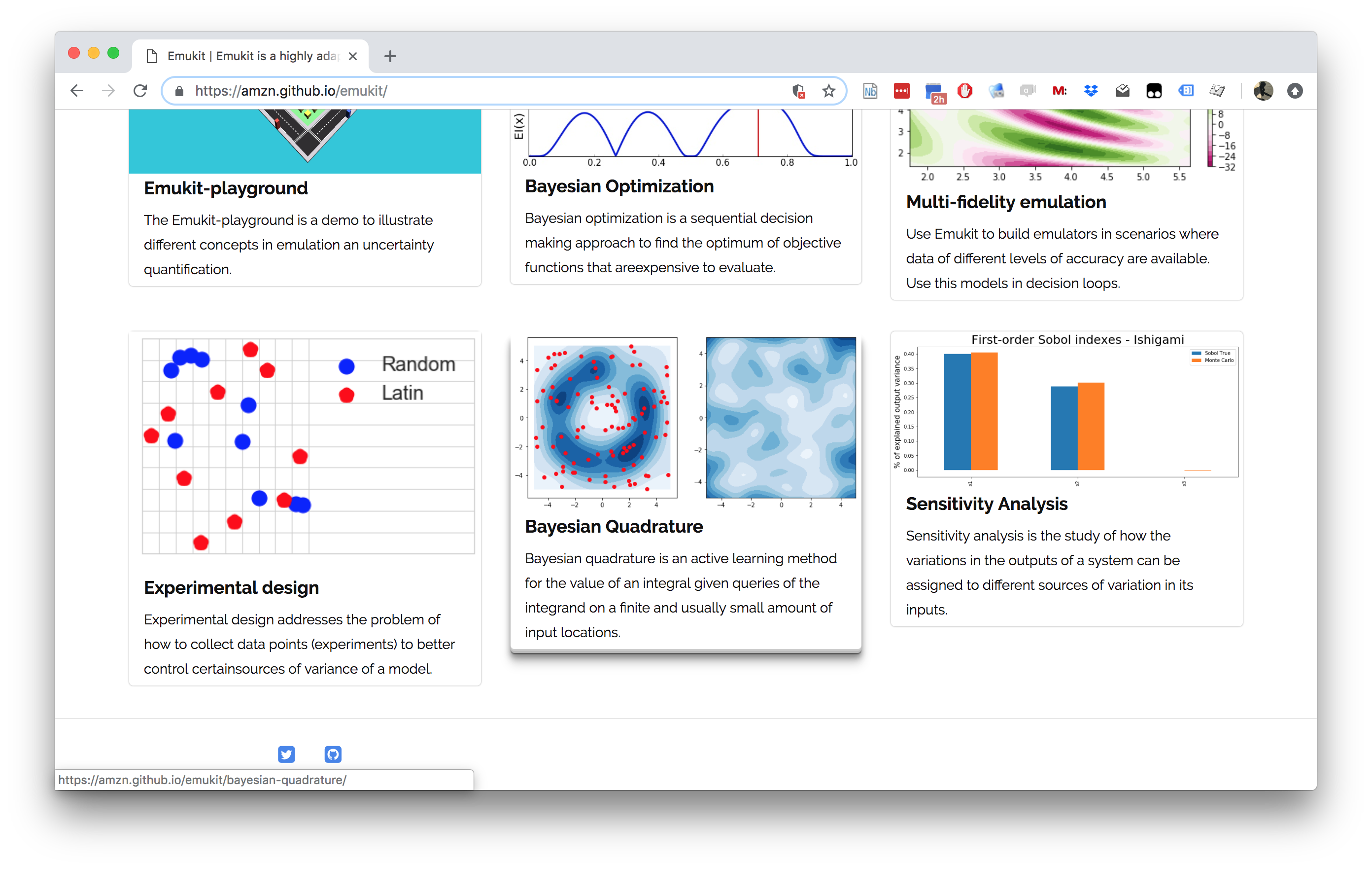
Emukit

  • Work by Javier Gonzalez, Andrei Paleyes, Mark Pullin, Maren Mahsereci, Alex Gessner, Aaron Klein.
  • Available on Github
  • Example sensitivity notebook.

Emukit Software

  • Multi-fidelity emulation: build surrogate models for multiple sources of information;
  • Bayesian optimisation: optimise physical experiments and tune parameters ML algorithms;
  • Experimental design/Active learning: design experiments and perform active learning with ML models;
  • Sensitivity analysis: analyse the influence of inputs on the outputs
  • Bayesian quadrature: compute integrals of functions that are expensive to evaluate.

Conclusion

  • Artificial Intelligence and Data Science are fundamentally different.

  • In one you are dealing with data collected by happenstance.

  • In the other you are trying to build systems in the real world, often by actively collecting data.

  • Our approaches to systems design are building powerful machines that will be deployed in evolving environments.

Thanks!

References

Lawrence, N.D., 2017. Living together: Mind and machine intelligence. arXiv.

Taigman, Y., Yang, M., Ranzato, M., Wolf, L., 2014. DeepFace: Closing the gap to human-level performance in face verification, in: Proceedings of the IEEE Computer Society Conference on Computer Vision and Pattern Recognition. https://doi.org/10.1109/CVPR.2014.220