Data First Culture
Getting the Information Ecosystem Ready for the AI Revolution
Advanced Leadership Programme, Judge Business School, University of Cambridge
|
|
|

|
|
|
bits/min
|
billions
|
2000
|
6
|
|
billion
calculations/s |
~100
|
a billion
|
a billion
|
|
embodiment
|
20 minutes
|
5 billion years
|
15 trillion years
|
.
Mathematical Statistics

‘Mathematical Data Science’

DeepFace
Outline of the DeepFace architecture. A front-end of a single convolution-pooling-convolution filtering on the rectified input, followed by three locally-connected layers and two fully-connected layers. Color illustrates feature maps produced at each layer. The net includes more than 120 million parameters, where more than 95% come from the local and fully connected.
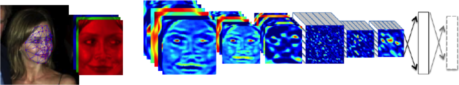
Source: DeepFace (Taigman et al., 2014)
Deep Learning as Pinball

Supply Chain
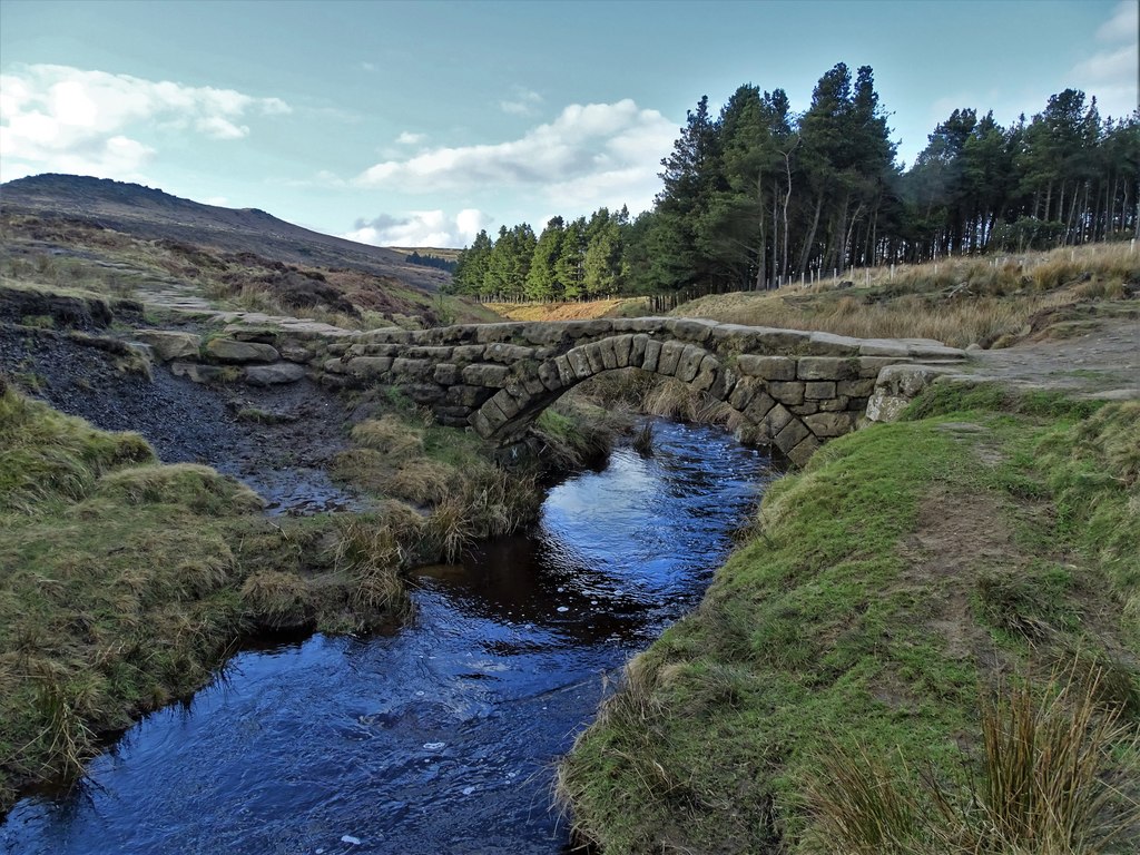
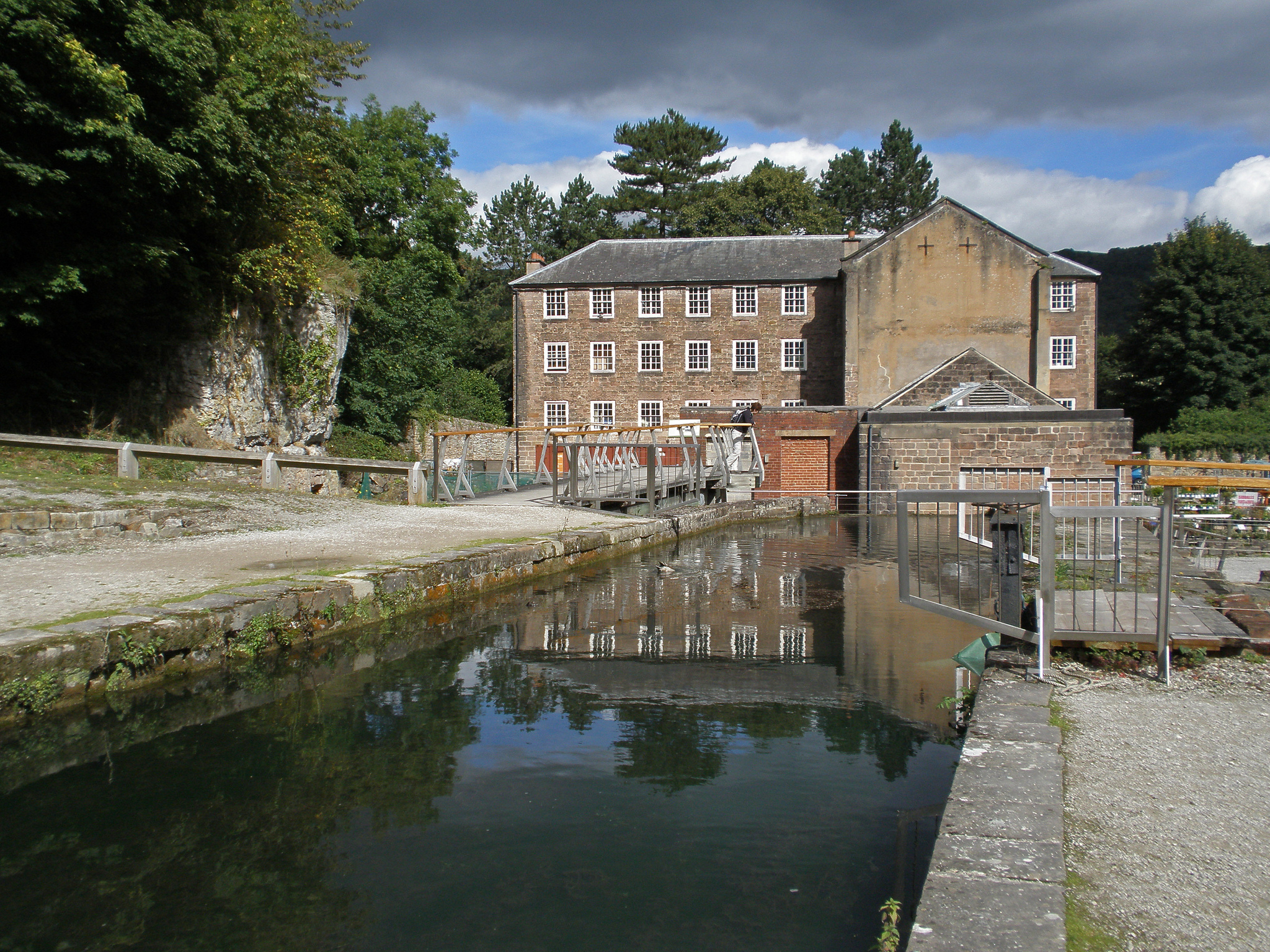
Cromford

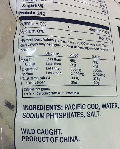
Deep Freeze

Deep Freeze
Data Readiness Levels

https://arxiv.org/pdf/1705.02245.pdf Data Readiness Levels (Lawrence, 2017)