AI and Data Science

Neil D. Lawrence

$$\newcommand{\tk}[1]{} \newcommand{\Amatrix}{\mathbf{A}} \newcommand{\KL}[2]{\text{KL}\left( #1\,\|\,#2 \right)} \newcommand{\Kaast}{\kernelMatrix_{\mathbf{ \ast}\mathbf{ \ast}}} \newcommand{\Kastu}{\kernelMatrix_{\mathbf{ \ast} \inducingVector}} \newcommand{\Kff}{\kernelMatrix_{\mappingFunctionVector \mappingFunctionVector}} \newcommand{\Kfu}{\kernelMatrix_{\mappingFunctionVector \inducingVector}} \newcommand{\Kuast}{\kernelMatrix_{\inducingVector \bf\ast}} \newcommand{\Kuf}{\kernelMatrix_{\inducingVector \mappingFunctionVector}} \newcommand{\Kuu}{\kernelMatrix_{\inducingVector \inducingVector}} \newcommand{\Kuui}{\Kuu^{-1}} \newcommand{\Qaast}{\mathbf{Q}_{\bf \ast \ast}} \newcommand{\Qastf}{\mathbf{Q}_{\ast \mappingFunction}} \newcommand{\Qfast}{\mathbf{Q}_{\mappingFunctionVector \bf \ast}} \newcommand{\Qff}{\mathbf{Q}_{\mappingFunctionVector \mappingFunctionVector}} \newcommand{\aMatrix}{\mathbf{A}} \newcommand{\aScalar}{a} \newcommand{\aVector}{\mathbf{a}} \newcommand{\acceleration}{a} \newcommand{\bMatrix}{\mathbf{B}} \newcommand{\bScalar}{b} \newcommand{\bVector}{\mathbf{b}} \newcommand{\basisFunc}{\phi} \newcommand{\basisFuncVector}{\boldsymbol{ \basisFunc}} \newcommand{\basisFunction}{\phi} \newcommand{\basisLocation}{\mu} \newcommand{\basisMatrix}{\boldsymbol{ \Phi}} \newcommand{\basisScalar}{\basisFunction} \newcommand{\basisVector}{\boldsymbol{ \basisFunction}} \newcommand{\activationFunction}{\phi} \newcommand{\activationMatrix}{\boldsymbol{ \Phi}} \newcommand{\activationScalar}{\basisFunction} \newcommand{\activationVector}{\boldsymbol{ \basisFunction}} \newcommand{\bigO}{\mathcal{O}} \newcommand{\binomProb}{\pi} \newcommand{\cMatrix}{\mathbf{C}} \newcommand{\cbasisMatrix}{\hat{\boldsymbol{ \Phi}}} \newcommand{\cdataMatrix}{\hat{\dataMatrix}} \newcommand{\cdataScalar}{\hat{\dataScalar}} \newcommand{\cdataVector}{\hat{\dataVector}} \newcommand{\centeredKernelMatrix}{\mathbf{ \MakeUppercase{\centeredKernelScalar}}} \newcommand{\centeredKernelScalar}{b} \newcommand{\centeredKernelVector}{\centeredKernelScalar} \newcommand{\centeringMatrix}{\mathbf{H}} \newcommand{\chiSquaredDist}[2]{\chi_{#1}^{2}\left(#2\right)} \newcommand{\chiSquaredSamp}[1]{\chi_{#1}^{2}} \newcommand{\conditionalCovariance}{\boldsymbol{ \Sigma}} \newcommand{\coregionalizationMatrix}{\mathbf{B}} \newcommand{\coregionalizationScalar}{b} \newcommand{\coregionalizationVector}{\mathbf{ \coregionalizationScalar}} \newcommand{\covDist}[2]{\text{cov}_{#2}\left(#1\right)} \newcommand{\covSamp}[1]{\text{cov}\left(#1\right)} \newcommand{\covarianceScalar}{c} \newcommand{\covarianceVector}{\mathbf{ \covarianceScalar}} \newcommand{\covarianceMatrix}{\mathbf{C}} \newcommand{\covarianceMatrixTwo}{\boldsymbol{ \Sigma}} \newcommand{\croupierScalar}{s} \newcommand{\croupierVector}{\mathbf{ \croupierScalar}} \newcommand{\croupierMatrix}{\mathbf{ \MakeUppercase{\croupierScalar}}} \newcommand{\dataDim}{p} \newcommand{\dataIndex}{i} \newcommand{\dataIndexTwo}{j} \newcommand{\dataMatrix}{\mathbf{Y}} \newcommand{\dataScalar}{y} \newcommand{\dataSet}{\mathcal{D}} \newcommand{\dataStd}{\sigma} \newcommand{\dataVector}{\mathbf{ \dataScalar}} \newcommand{\decayRate}{d} \newcommand{\degreeMatrix}{\mathbf{ \MakeUppercase{\degreeScalar}}} \newcommand{\degreeScalar}{d} \newcommand{\degreeVector}{\mathbf{ \degreeScalar}} \newcommand{\diag}[1]{\text{diag}\left(#1\right)} \newcommand{\diagonalMatrix}{\mathbf{D}} \newcommand{\diff}[2]{\frac{\text{d}#1}{\text{d}#2}} \newcommand{\diffTwo}[2]{\frac{\text{d}^2#1}{\text{d}#2^2}} \newcommand{\displacement}{x} \newcommand{\displacementVector}{\textbf{\displacement}} \newcommand{\distanceMatrix}{\mathbf{ \MakeUppercase{\distanceScalar}}} \newcommand{\distanceScalar}{d} \newcommand{\distanceVector}{\mathbf{ \distanceScalar}} \newcommand{\eigenvaltwo}{\ell} \newcommand{\eigenvaltwoMatrix}{\mathbf{L}} \newcommand{\eigenvaltwoVector}{\mathbf{l}} \newcommand{\eigenvalue}{\lambda} \newcommand{\eigenvalueMatrix}{\boldsymbol{ \Lambda}} \newcommand{\eigenvalueVector}{\boldsymbol{ \lambda}} \newcommand{\eigenvector}{\mathbf{ \eigenvectorScalar}} \newcommand{\eigenvectorMatrix}{\mathbf{U}} \newcommand{\eigenvectorScalar}{u} \newcommand{\eigenvectwo}{\mathbf{v}} \newcommand{\eigenvectwoMatrix}{\mathbf{V}} \newcommand{\eigenvectwoScalar}{v} \newcommand{\entropy}[1]{\mathcal{H}\left(#1\right)} \newcommand{\errorFunction}{E} \newcommand{\expDist}[2]{\left\langle#1\right\rangle_{#2}} \newcommand{\expSamp}[1]{\left\langle#1\right\rangle} \newcommand{\expectation}[1]{\left\langle #1 \right\rangle } \newcommand{\expectationDist}[2]{\left\langle #1 \right\rangle _{#2}} \newcommand{\expectedDistanceMatrix}{\mathcal{D}} \newcommand{\eye}{\mathbf{I}} \newcommand{\fantasyDim}{r} \newcommand{\fantasyMatrix}{\mathbf{ \MakeUppercase{\fantasyScalar}}} \newcommand{\fantasyScalar}{z} \newcommand{\fantasyVector}{\mathbf{ \fantasyScalar}} \newcommand{\featureStd}{\varsigma} \newcommand{\gammaCdf}[3]{\mathcal{GAMMA CDF}\left(#1|#2,#3\right)} \newcommand{\gammaDist}[3]{\mathcal{G}\left(#1|#2,#3\right)} \newcommand{\gammaSamp}[2]{\mathcal{G}\left(#1,#2\right)} \newcommand{\gaussianDist}[3]{\mathcal{N}\left(#1|#2,#3\right)} \newcommand{\gaussianSamp}[2]{\mathcal{N}\left(#1,#2\right)} \newcommand{\uniformDist}[3]{\mathcal{U}\left(#1|#2,#3\right)} \newcommand{\uniformSamp}[2]{\mathcal{U}\left(#1,#2\right)} \newcommand{\given}{|} \newcommand{\half}{\frac{1}{2}} \newcommand{\heaviside}{H} \newcommand{\hiddenMatrix}{\mathbf{ \MakeUppercase{\hiddenScalar}}} \newcommand{\hiddenScalar}{h} \newcommand{\hiddenVector}{\mathbf{ \hiddenScalar}} \newcommand{\identityMatrix}{\eye} \newcommand{\inducingInputScalar}{z} \newcommand{\inducingInputVector}{\mathbf{ \inducingInputScalar}} \newcommand{\inducingInputMatrix}{\mathbf{Z}} \newcommand{\inducingScalar}{u} \newcommand{\inducingVector}{\mathbf{ \inducingScalar}} \newcommand{\inducingMatrix}{\mathbf{U}} \newcommand{\inlineDiff}[2]{\text{d}#1/\text{d}#2} \newcommand{\inputDim}{q} \newcommand{\inputMatrix}{\mathbf{X}} \newcommand{\inputScalar}{x} \newcommand{\inputSpace}{\mathcal{X}} \newcommand{\inputVals}{\inputVector} \newcommand{\inputVector}{\mathbf{ \inputScalar}} \newcommand{\iterNum}{k} \newcommand{\kernel}{\kernelScalar} \newcommand{\kernelMatrix}{\mathbf{K}} \newcommand{\kernelScalar}{k} \newcommand{\kernelVector}{\mathbf{ \kernelScalar}} \newcommand{\kff}{\kernelScalar_{\mappingFunction \mappingFunction}} \newcommand{\kfu}{\kernelVector_{\mappingFunction \inducingScalar}} \newcommand{\kuf}{\kernelVector_{\inducingScalar \mappingFunction}} \newcommand{\kuu}{\kernelVector_{\inducingScalar \inducingScalar}} \newcommand{\lagrangeMultiplier}{\lambda} \newcommand{\lagrangeMultiplierMatrix}{\boldsymbol{ \Lambda}} \newcommand{\lagrangian}{L} \newcommand{\laplacianFactor}{\mathbf{ \MakeUppercase{\laplacianFactorScalar}}} \newcommand{\laplacianFactorScalar}{m} \newcommand{\laplacianFactorVector}{\mathbf{ \laplacianFactorScalar}} \newcommand{\laplacianMatrix}{\mathbf{L}} \newcommand{\laplacianScalar}{\ell} \newcommand{\laplacianVector}{\mathbf{ \ell}} \newcommand{\latentDim}{q} \newcommand{\latentDistanceMatrix}{\boldsymbol{ \Delta}} \newcommand{\latentDistanceScalar}{\delta} \newcommand{\latentDistanceVector}{\boldsymbol{ \delta}} \newcommand{\latentForce}{f} \newcommand{\latentFunction}{u} \newcommand{\latentFunctionVector}{\mathbf{ \latentFunction}} \newcommand{\latentFunctionMatrix}{\mathbf{ \MakeUppercase{\latentFunction}}} \newcommand{\latentIndex}{j} \newcommand{\latentScalar}{z} \newcommand{\latentVector}{\mathbf{ \latentScalar}} \newcommand{\latentMatrix}{\mathbf{Z}} \newcommand{\learnRate}{\eta} \newcommand{\lengthScale}{\ell} \newcommand{\rbfWidth}{\ell} \newcommand{\likelihoodBound}{\mathcal{L}} \newcommand{\likelihoodFunction}{L} \newcommand{\locationScalar}{\mu} \newcommand{\locationVector}{\boldsymbol{ \locationScalar}} \newcommand{\locationMatrix}{\mathbf{M}} \newcommand{\variance}[1]{\text{var}\left( #1 \right)} \newcommand{\mappingFunction}{f} \newcommand{\mappingFunctionMatrix}{\mathbf{F}} \newcommand{\mappingFunctionTwo}{g} \newcommand{\mappingFunctionTwoMatrix}{\mathbf{G}} \newcommand{\mappingFunctionTwoVector}{\mathbf{ \mappingFunctionTwo}} \newcommand{\mappingFunctionVector}{\mathbf{ \mappingFunction}} \newcommand{\scaleScalar}{s} \newcommand{\mappingScalar}{w} \newcommand{\mappingVector}{\mathbf{ \mappingScalar}} \newcommand{\mappingMatrix}{\mathbf{W}} \newcommand{\mappingScalarTwo}{v} \newcommand{\mappingVectorTwo}{\mathbf{ \mappingScalarTwo}} \newcommand{\mappingMatrixTwo}{\mathbf{V}} \newcommand{\maxIters}{K} \newcommand{\meanMatrix}{\mathbf{M}} \newcommand{\meanScalar}{\mu} \newcommand{\meanTwoMatrix}{\mathbf{M}} \newcommand{\meanTwoScalar}{m} \newcommand{\meanTwoVector}{\mathbf{ \meanTwoScalar}} \newcommand{\meanVector}{\boldsymbol{ \meanScalar}} \newcommand{\mrnaConcentration}{m} \newcommand{\naturalFrequency}{\omega} \newcommand{\neighborhood}[1]{\mathcal{N}\left( #1 \right)} \newcommand{\neilurl}{http://inverseprobability.com/} \newcommand{\noiseMatrix}{\boldsymbol{ E}} \newcommand{\noiseScalar}{\epsilon} \newcommand{\noiseVector}{\boldsymbol{ \epsilon}} \newcommand{\noiseStd}{\sigma} \newcommand{\norm}[1]{\left\Vert #1 \right\Vert} \newcommand{\normalizedLaplacianMatrix}{\hat{\mathbf{L}}} \newcommand{\normalizedLaplacianScalar}{\hat{\ell}} \newcommand{\normalizedLaplacianVector}{\hat{\mathbf{ \ell}}} \newcommand{\numActive}{m} \newcommand{\numBasisFunc}{m} \newcommand{\numComponents}{m} \newcommand{\numComps}{K} \newcommand{\numData}{n} \newcommand{\numFeatures}{K} \newcommand{\numHidden}{h} \newcommand{\numInducing}{m} \newcommand{\numLayers}{\ell} \newcommand{\numNeighbors}{K} \newcommand{\numSequences}{s} \newcommand{\numSuccess}{s} \newcommand{\numTasks}{m} \newcommand{\numTime}{T} \newcommand{\numTrials}{S} \newcommand{\outputIndex}{j} \newcommand{\paramVector}{\boldsymbol{ \theta}} \newcommand{\parameterMatrix}{\boldsymbol{ \Theta}} \newcommand{\parameterScalar}{\theta} \newcommand{\parameterVector}{\boldsymbol{ \parameterScalar}} \newcommand{\partDiff}[2]{\frac{\partial#1}{\partial#2}} \newcommand{\precisionScalar}{j} \newcommand{\precisionVector}{\mathbf{ \precisionScalar}} \newcommand{\precisionMatrix}{\mathbf{J}} \newcommand{\pseudotargetScalar}{\widetilde{y}} \newcommand{\pseudotargetVector}{\mathbf{ \pseudotargetScalar}} \newcommand{\pseudotargetMatrix}{\mathbf{ \widetilde{Y}}} \newcommand{\rank}[1]{\text{rank}\left(#1\right)} \newcommand{\rayleighDist}[2]{\mathcal{R}\left(#1|#2\right)} \newcommand{\rayleighSamp}[1]{\mathcal{R}\left(#1\right)} \newcommand{\responsibility}{r} \newcommand{\rotationScalar}{r} \newcommand{\rotationVector}{\mathbf{ \rotationScalar}} \newcommand{\rotationMatrix}{\mathbf{R}} \newcommand{\sampleCovScalar}{s} \newcommand{\sampleCovVector}{\mathbf{ \sampleCovScalar}} \newcommand{\sampleCovMatrix}{\mathbf{s}} \newcommand{\scalarProduct}[2]{\left\langle{#1},{#2}\right\rangle} \newcommand{\sign}[1]{\text{sign}\left(#1\right)} \newcommand{\sigmoid}[1]{\sigma\left(#1\right)} \newcommand{\singularvalue}{\ell} \newcommand{\singularvalueMatrix}{\mathbf{L}} \newcommand{\singularvalueVector}{\mathbf{l}} \newcommand{\sorth}{\mathbf{u}} \newcommand{\spar}{\lambda} \newcommand{\trace}[1]{\text{tr}\left(#1\right)} \newcommand{\BasalRate}{B} \newcommand{\DampingCoefficient}{C} \newcommand{\DecayRate}{D} \newcommand{\Displacement}{X} \newcommand{\LatentForce}{F} \newcommand{\Mass}{M} \newcommand{\Sensitivity}{S} \newcommand{\basalRate}{b} \newcommand{\dampingCoefficient}{c} \newcommand{\mass}{m} \newcommand{\sensitivity}{s} \newcommand{\springScalar}{\kappa} \newcommand{\springVector}{\boldsymbol{ \kappa}} \newcommand{\springMatrix}{\boldsymbol{ \mathcal{K}}} \newcommand{\tfConcentration}{p} \newcommand{\tfDecayRate}{\delta} \newcommand{\tfMrnaConcentration}{f} \newcommand{\tfVector}{\mathbf{ \tfConcentration}} \newcommand{\velocity}{v} \newcommand{\sufficientStatsScalar}{g} \newcommand{\sufficientStatsVector}{\mathbf{ \sufficientStatsScalar}} \newcommand{\sufficientStatsMatrix}{\mathbf{G}} \newcommand{\switchScalar}{s} \newcommand{\switchVector}{\mathbf{ \switchScalar}} \newcommand{\switchMatrix}{\mathbf{S}} \newcommand{\tr}[1]{\text{tr}\left(#1\right)} \newcommand{\loneNorm}[1]{\left\Vert #1 \right\Vert_1} \newcommand{\ltwoNorm}[1]{\left\Vert #1 \right\Vert_2} \newcommand{\onenorm}[1]{\left\vert#1\right\vert_1} \newcommand{\twonorm}[1]{\left\Vert #1 \right\Vert} \newcommand{\vScalar}{v} \newcommand{\vVector}{\mathbf{v}} \newcommand{\vMatrix}{\mathbf{V}} \newcommand{\varianceDist}[2]{\text{var}_{#2}\left( #1 \right)} \newcommand{\vecb}[1]{\left(#1\right):} \newcommand{\weightScalar}{w} \newcommand{\weightVector}{\mathbf{ \weightScalar}} \newcommand{\weightMatrix}{\mathbf{W}} \newcommand{\weightedAdjacencyMatrix}{\mathbf{A}} \newcommand{\weightedAdjacencyScalar}{a} \newcommand{\weightedAdjacencyVector}{\mathbf{ \weightedAdjacencyScalar}} \newcommand{\onesVector}{\mathbf{1}} \newcommand{\zerosVector}{\mathbf{0}} $$

at Autumn Data Science School, Cambridge on Sep 22, 2020 [reveal]

Neil D. Lawrence, University of Cambridge

Abstract

Waves of automation have driven human advance, and each wave requires humans to The promise of AI is to launch new systems of automated intellectual endeavour that will be the first systems to adapt to us. In reality, the systems we have will not achieve this, and it is the biological sciences that teach us this lesson most starkly. In this talk I will review some of the successes and challenges of AI and its deployment and propose practical visions for the future based on approaches that have worked in the past.

$$\newcommand{\tk}[1]{} \newcommand{\Amatrix}{\mathbf{A}} \newcommand{\KL}[2]{\text{KL}\left( #1\,\|\,#2 \right)} \newcommand{\Kaast}{\kernelMatrix_{\mathbf{ \ast}\mathbf{ \ast}}} \newcommand{\Kastu}{\kernelMatrix_{\mathbf{ \ast} \inducingVector}} \newcommand{\Kff}{\kernelMatrix_{\mappingFunctionVector \mappingFunctionVector}} \newcommand{\Kfu}{\kernelMatrix_{\mappingFunctionVector \inducingVector}} \newcommand{\Kuast}{\kernelMatrix_{\inducingVector \bf\ast}} \newcommand{\Kuf}{\kernelMatrix_{\inducingVector \mappingFunctionVector}} \newcommand{\Kuu}{\kernelMatrix_{\inducingVector \inducingVector}} \newcommand{\Kuui}{\Kuu^{-1}} \newcommand{\Qaast}{\mathbf{Q}_{\bf \ast \ast}} \newcommand{\Qastf}{\mathbf{Q}_{\ast \mappingFunction}} \newcommand{\Qfast}{\mathbf{Q}_{\mappingFunctionVector \bf \ast}} \newcommand{\Qff}{\mathbf{Q}_{\mappingFunctionVector \mappingFunctionVector}} \newcommand{\aMatrix}{\mathbf{A}} \newcommand{\aScalar}{a} \newcommand{\aVector}{\mathbf{a}} \newcommand{\acceleration}{a} \newcommand{\bMatrix}{\mathbf{B}} \newcommand{\bScalar}{b} \newcommand{\bVector}{\mathbf{b}} \newcommand{\basisFunc}{\phi} \newcommand{\basisFuncVector}{\boldsymbol{ \basisFunc}} \newcommand{\basisFunction}{\phi} \newcommand{\basisLocation}{\mu} \newcommand{\basisMatrix}{\boldsymbol{ \Phi}} \newcommand{\basisScalar}{\basisFunction} \newcommand{\basisVector}{\boldsymbol{ \basisFunction}} \newcommand{\activationFunction}{\phi} \newcommand{\activationMatrix}{\boldsymbol{ \Phi}} \newcommand{\activationScalar}{\basisFunction} \newcommand{\activationVector}{\boldsymbol{ \basisFunction}} \newcommand{\bigO}{\mathcal{O}} \newcommand{\binomProb}{\pi} \newcommand{\cMatrix}{\mathbf{C}} \newcommand{\cbasisMatrix}{\hat{\boldsymbol{ \Phi}}} \newcommand{\cdataMatrix}{\hat{\dataMatrix}} \newcommand{\cdataScalar}{\hat{\dataScalar}} \newcommand{\cdataVector}{\hat{\dataVector}} \newcommand{\centeredKernelMatrix}{\mathbf{ \MakeUppercase{\centeredKernelScalar}}} \newcommand{\centeredKernelScalar}{b} \newcommand{\centeredKernelVector}{\centeredKernelScalar} \newcommand{\centeringMatrix}{\mathbf{H}} \newcommand{\chiSquaredDist}[2]{\chi_{#1}^{2}\left(#2\right)} \newcommand{\chiSquaredSamp}[1]{\chi_{#1}^{2}} \newcommand{\conditionalCovariance}{\boldsymbol{ \Sigma}} \newcommand{\coregionalizationMatrix}{\mathbf{B}} \newcommand{\coregionalizationScalar}{b} \newcommand{\coregionalizationVector}{\mathbf{ \coregionalizationScalar}} \newcommand{\covDist}[2]{\text{cov}_{#2}\left(#1\right)} \newcommand{\covSamp}[1]{\text{cov}\left(#1\right)} \newcommand{\covarianceScalar}{c} \newcommand{\covarianceVector}{\mathbf{ \covarianceScalar}} \newcommand{\covarianceMatrix}{\mathbf{C}} \newcommand{\covarianceMatrixTwo}{\boldsymbol{ \Sigma}} \newcommand{\croupierScalar}{s} \newcommand{\croupierVector}{\mathbf{ \croupierScalar}} \newcommand{\croupierMatrix}{\mathbf{ \MakeUppercase{\croupierScalar}}} \newcommand{\dataDim}{p} \newcommand{\dataIndex}{i} \newcommand{\dataIndexTwo}{j} \newcommand{\dataMatrix}{\mathbf{Y}} \newcommand{\dataScalar}{y} \newcommand{\dataSet}{\mathcal{D}} \newcommand{\dataStd}{\sigma} \newcommand{\dataVector}{\mathbf{ \dataScalar}} \newcommand{\decayRate}{d} \newcommand{\degreeMatrix}{\mathbf{ \MakeUppercase{\degreeScalar}}} \newcommand{\degreeScalar}{d} \newcommand{\degreeVector}{\mathbf{ \degreeScalar}} \newcommand{\diag}[1]{\text{diag}\left(#1\right)} \newcommand{\diagonalMatrix}{\mathbf{D}} \newcommand{\diff}[2]{\frac{\text{d}#1}{\text{d}#2}} \newcommand{\diffTwo}[2]{\frac{\text{d}^2#1}{\text{d}#2^2}} \newcommand{\displacement}{x} \newcommand{\displacementVector}{\textbf{\displacement}} \newcommand{\distanceMatrix}{\mathbf{ \MakeUppercase{\distanceScalar}}} \newcommand{\distanceScalar}{d} \newcommand{\distanceVector}{\mathbf{ \distanceScalar}} \newcommand{\eigenvaltwo}{\ell} \newcommand{\eigenvaltwoMatrix}{\mathbf{L}} \newcommand{\eigenvaltwoVector}{\mathbf{l}} \newcommand{\eigenvalue}{\lambda} \newcommand{\eigenvalueMatrix}{\boldsymbol{ \Lambda}} \newcommand{\eigenvalueVector}{\boldsymbol{ \lambda}} \newcommand{\eigenvector}{\mathbf{ \eigenvectorScalar}} \newcommand{\eigenvectorMatrix}{\mathbf{U}} \newcommand{\eigenvectorScalar}{u} \newcommand{\eigenvectwo}{\mathbf{v}} \newcommand{\eigenvectwoMatrix}{\mathbf{V}} \newcommand{\eigenvectwoScalar}{v} \newcommand{\entropy}[1]{\mathcal{H}\left(#1\right)} \newcommand{\errorFunction}{E} \newcommand{\expDist}[2]{\left\langle#1\right\rangle_{#2}} \newcommand{\expSamp}[1]{\left\langle#1\right\rangle} \newcommand{\expectation}[1]{\left\langle #1 \right\rangle } \newcommand{\expectationDist}[2]{\left\langle #1 \right\rangle _{#2}} \newcommand{\expectedDistanceMatrix}{\mathcal{D}} \newcommand{\eye}{\mathbf{I}} \newcommand{\fantasyDim}{r} \newcommand{\fantasyMatrix}{\mathbf{ \MakeUppercase{\fantasyScalar}}} \newcommand{\fantasyScalar}{z} \newcommand{\fantasyVector}{\mathbf{ \fantasyScalar}} \newcommand{\featureStd}{\varsigma} \newcommand{\gammaCdf}[3]{\mathcal{GAMMA CDF}\left(#1|#2,#3\right)} \newcommand{\gammaDist}[3]{\mathcal{G}\left(#1|#2,#3\right)} \newcommand{\gammaSamp}[2]{\mathcal{G}\left(#1,#2\right)} \newcommand{\gaussianDist}[3]{\mathcal{N}\left(#1|#2,#3\right)} \newcommand{\gaussianSamp}[2]{\mathcal{N}\left(#1,#2\right)} \newcommand{\uniformDist}[3]{\mathcal{U}\left(#1|#2,#3\right)} \newcommand{\uniformSamp}[2]{\mathcal{U}\left(#1,#2\right)} \newcommand{\given}{|} \newcommand{\half}{\frac{1}{2}} \newcommand{\heaviside}{H} \newcommand{\hiddenMatrix}{\mathbf{ \MakeUppercase{\hiddenScalar}}} \newcommand{\hiddenScalar}{h} \newcommand{\hiddenVector}{\mathbf{ \hiddenScalar}} \newcommand{\identityMatrix}{\eye} \newcommand{\inducingInputScalar}{z} \newcommand{\inducingInputVector}{\mathbf{ \inducingInputScalar}} \newcommand{\inducingInputMatrix}{\mathbf{Z}} \newcommand{\inducingScalar}{u} \newcommand{\inducingVector}{\mathbf{ \inducingScalar}} \newcommand{\inducingMatrix}{\mathbf{U}} \newcommand{\inlineDiff}[2]{\text{d}#1/\text{d}#2} \newcommand{\inputDim}{q} \newcommand{\inputMatrix}{\mathbf{X}} \newcommand{\inputScalar}{x} \newcommand{\inputSpace}{\mathcal{X}} \newcommand{\inputVals}{\inputVector} \newcommand{\inputVector}{\mathbf{ \inputScalar}} \newcommand{\iterNum}{k} \newcommand{\kernel}{\kernelScalar} \newcommand{\kernelMatrix}{\mathbf{K}} \newcommand{\kernelScalar}{k} \newcommand{\kernelVector}{\mathbf{ \kernelScalar}} \newcommand{\kff}{\kernelScalar_{\mappingFunction \mappingFunction}} \newcommand{\kfu}{\kernelVector_{\mappingFunction \inducingScalar}} \newcommand{\kuf}{\kernelVector_{\inducingScalar \mappingFunction}} \newcommand{\kuu}{\kernelVector_{\inducingScalar \inducingScalar}} \newcommand{\lagrangeMultiplier}{\lambda} \newcommand{\lagrangeMultiplierMatrix}{\boldsymbol{ \Lambda}} \newcommand{\lagrangian}{L} \newcommand{\laplacianFactor}{\mathbf{ \MakeUppercase{\laplacianFactorScalar}}} \newcommand{\laplacianFactorScalar}{m} \newcommand{\laplacianFactorVector}{\mathbf{ \laplacianFactorScalar}} \newcommand{\laplacianMatrix}{\mathbf{L}} \newcommand{\laplacianScalar}{\ell} \newcommand{\laplacianVector}{\mathbf{ \ell}} \newcommand{\latentDim}{q} \newcommand{\latentDistanceMatrix}{\boldsymbol{ \Delta}} \newcommand{\latentDistanceScalar}{\delta} \newcommand{\latentDistanceVector}{\boldsymbol{ \delta}} \newcommand{\latentForce}{f} \newcommand{\latentFunction}{u} \newcommand{\latentFunctionVector}{\mathbf{ \latentFunction}} \newcommand{\latentFunctionMatrix}{\mathbf{ \MakeUppercase{\latentFunction}}} \newcommand{\latentIndex}{j} \newcommand{\latentScalar}{z} \newcommand{\latentVector}{\mathbf{ \latentScalar}} \newcommand{\latentMatrix}{\mathbf{Z}} \newcommand{\learnRate}{\eta} \newcommand{\lengthScale}{\ell} \newcommand{\rbfWidth}{\ell} \newcommand{\likelihoodBound}{\mathcal{L}} \newcommand{\likelihoodFunction}{L} \newcommand{\locationScalar}{\mu} \newcommand{\locationVector}{\boldsymbol{ \locationScalar}} \newcommand{\locationMatrix}{\mathbf{M}} \newcommand{\variance}[1]{\text{var}\left( #1 \right)} \newcommand{\mappingFunction}{f} \newcommand{\mappingFunctionMatrix}{\mathbf{F}} \newcommand{\mappingFunctionTwo}{g} \newcommand{\mappingFunctionTwoMatrix}{\mathbf{G}} \newcommand{\mappingFunctionTwoVector}{\mathbf{ \mappingFunctionTwo}} \newcommand{\mappingFunctionVector}{\mathbf{ \mappingFunction}} \newcommand{\scaleScalar}{s} \newcommand{\mappingScalar}{w} \newcommand{\mappingVector}{\mathbf{ \mappingScalar}} \newcommand{\mappingMatrix}{\mathbf{W}} \newcommand{\mappingScalarTwo}{v} \newcommand{\mappingVectorTwo}{\mathbf{ \mappingScalarTwo}} \newcommand{\mappingMatrixTwo}{\mathbf{V}} \newcommand{\maxIters}{K} \newcommand{\meanMatrix}{\mathbf{M}} \newcommand{\meanScalar}{\mu} \newcommand{\meanTwoMatrix}{\mathbf{M}} \newcommand{\meanTwoScalar}{m} \newcommand{\meanTwoVector}{\mathbf{ \meanTwoScalar}} \newcommand{\meanVector}{\boldsymbol{ \meanScalar}} \newcommand{\mrnaConcentration}{m} \newcommand{\naturalFrequency}{\omega} \newcommand{\neighborhood}[1]{\mathcal{N}\left( #1 \right)} \newcommand{\neilurl}{http://inverseprobability.com/} \newcommand{\noiseMatrix}{\boldsymbol{ E}} \newcommand{\noiseScalar}{\epsilon} \newcommand{\noiseVector}{\boldsymbol{ \epsilon}} \newcommand{\noiseStd}{\sigma} \newcommand{\norm}[1]{\left\Vert #1 \right\Vert} \newcommand{\normalizedLaplacianMatrix}{\hat{\mathbf{L}}} \newcommand{\normalizedLaplacianScalar}{\hat{\ell}} \newcommand{\normalizedLaplacianVector}{\hat{\mathbf{ \ell}}} \newcommand{\numActive}{m} \newcommand{\numBasisFunc}{m} \newcommand{\numComponents}{m} \newcommand{\numComps}{K} \newcommand{\numData}{n} \newcommand{\numFeatures}{K} \newcommand{\numHidden}{h} \newcommand{\numInducing}{m} \newcommand{\numLayers}{\ell} \newcommand{\numNeighbors}{K} \newcommand{\numSequences}{s} \newcommand{\numSuccess}{s} \newcommand{\numTasks}{m} \newcommand{\numTime}{T} \newcommand{\numTrials}{S} \newcommand{\outputIndex}{j} \newcommand{\paramVector}{\boldsymbol{ \theta}} \newcommand{\parameterMatrix}{\boldsymbol{ \Theta}} \newcommand{\parameterScalar}{\theta} \newcommand{\parameterVector}{\boldsymbol{ \parameterScalar}} \newcommand{\partDiff}[2]{\frac{\partial#1}{\partial#2}} \newcommand{\precisionScalar}{j} \newcommand{\precisionVector}{\mathbf{ \precisionScalar}} \newcommand{\precisionMatrix}{\mathbf{J}} \newcommand{\pseudotargetScalar}{\widetilde{y}} \newcommand{\pseudotargetVector}{\mathbf{ \pseudotargetScalar}} \newcommand{\pseudotargetMatrix}{\mathbf{ \widetilde{Y}}} \newcommand{\rank}[1]{\text{rank}\left(#1\right)} \newcommand{\rayleighDist}[2]{\mathcal{R}\left(#1|#2\right)} \newcommand{\rayleighSamp}[1]{\mathcal{R}\left(#1\right)} \newcommand{\responsibility}{r} \newcommand{\rotationScalar}{r} \newcommand{\rotationVector}{\mathbf{ \rotationScalar}} \newcommand{\rotationMatrix}{\mathbf{R}} \newcommand{\sampleCovScalar}{s} \newcommand{\sampleCovVector}{\mathbf{ \sampleCovScalar}} \newcommand{\sampleCovMatrix}{\mathbf{s}} \newcommand{\scalarProduct}[2]{\left\langle{#1},{#2}\right\rangle} \newcommand{\sign}[1]{\text{sign}\left(#1\right)} \newcommand{\sigmoid}[1]{\sigma\left(#1\right)} \newcommand{\singularvalue}{\ell} \newcommand{\singularvalueMatrix}{\mathbf{L}} \newcommand{\singularvalueVector}{\mathbf{l}} \newcommand{\sorth}{\mathbf{u}} \newcommand{\spar}{\lambda} \newcommand{\trace}[1]{\text{tr}\left(#1\right)} \newcommand{\BasalRate}{B} \newcommand{\DampingCoefficient}{C} \newcommand{\DecayRate}{D} \newcommand{\Displacement}{X} \newcommand{\LatentForce}{F} \newcommand{\Mass}{M} \newcommand{\Sensitivity}{S} \newcommand{\basalRate}{b} \newcommand{\dampingCoefficient}{c} \newcommand{\mass}{m} \newcommand{\sensitivity}{s} \newcommand{\springScalar}{\kappa} \newcommand{\springVector}{\boldsymbol{ \kappa}} \newcommand{\springMatrix}{\boldsymbol{ \mathcal{K}}} \newcommand{\tfConcentration}{p} \newcommand{\tfDecayRate}{\delta} \newcommand{\tfMrnaConcentration}{f} \newcommand{\tfVector}{\mathbf{ \tfConcentration}} \newcommand{\velocity}{v} \newcommand{\sufficientStatsScalar}{g} \newcommand{\sufficientStatsVector}{\mathbf{ \sufficientStatsScalar}} \newcommand{\sufficientStatsMatrix}{\mathbf{G}} \newcommand{\switchScalar}{s} \newcommand{\switchVector}{\mathbf{ \switchScalar}} \newcommand{\switchMatrix}{\mathbf{S}} \newcommand{\tr}[1]{\text{tr}\left(#1\right)} \newcommand{\loneNorm}[1]{\left\Vert #1 \right\Vert_1} \newcommand{\ltwoNorm}[1]{\left\Vert #1 \right\Vert_2} \newcommand{\onenorm}[1]{\left\vert#1\right\vert_1} \newcommand{\twonorm}[1]{\left\Vert #1 \right\Vert} \newcommand{\vScalar}{v} \newcommand{\vVector}{\mathbf{v}} \newcommand{\vMatrix}{\mathbf{V}} \newcommand{\varianceDist}[2]{\text{var}_{#2}\left( #1 \right)} \newcommand{\vecb}[1]{\left(#1\right):} \newcommand{\weightScalar}{w} \newcommand{\weightVector}{\mathbf{ \weightScalar}} \newcommand{\weightMatrix}{\mathbf{W}} \newcommand{\weightedAdjacencyMatrix}{\mathbf{A}} \newcommand{\weightedAdjacencyScalar}{a} \newcommand{\weightedAdjacencyVector}{\mathbf{ \weightedAdjacencyScalar}} \newcommand{\onesVector}{\mathbf{1}} \newcommand{\zerosVector}{\mathbf{0}} $$

What is Machine Learning?

[edit]

What is machine learning? At its most basic level machine learning is a combination of

$$\text{data} + \text{model} \stackrel{\text{compute}}{\rightarrow} \text{prediction}$$

where data is our observations. They can be actively or passively acquired (meta-data). The model contains our assumptions, based on previous experience. That experience can be other data, it can come from transfer learning, or it can merely be our beliefs about the regularities of the universe. In humans our models include our inductive biases. The prediction is an action to be taken or a categorization or a quality score. The reason that machine learning has become a mainstay of artificial intelligence is the importance of predictions in artificial intelligence. The data and the model are combined through computation.

In practice we normally perform machine learning using two functions. To combine data with a model we typically make use of:

a prediction function a function which is used to make the predictions. It includes our beliefs about the regularities of the universe, our assumptions about how the world works, e.g. smoothness, spatial similarities, temporal similarities.

an objective function a function which defines the cost of misprediction. Typically it includes knowledge about the world’s generating processes (probabilistic objectives) or the costs we pay for mispredictions (empiricial risk minimization).

The combination of data and model through the prediction function and the objective function leads to a learning algorithm. The class of prediction functions and objective functions we can make use of is restricted by the algorithms they lead to. If the prediction function or the objective function are too complex, then it can be difficult to find an appropriate learning algorithm. Much of the acdemic field of machine learning is the quest for new learning algorithms that allow us to bring different types of models and data together.

A useful reference for state of the art in machine learning is the UK Royal Society Report, Machine Learning: Power and Promise of Computers that Learn by Example.

You can also check my post blog post on What is Machine Learning?..

Artificial Intelligence and Data Science

[edit]

Machine learning technologies have been the driver of two related, but distinct disciplines. The first is data science. Data science is an emerging field that arises from the fact that we now collect so much data by happenstance, rather than by experimental design. Classical statistics is the science of drawing conclusions from data, and to do so statistical experiments are carefully designed. In the modern era we collect so much data that there’s a desire to draw inferences directly from the data.

As well as machine learning, the field of data science draws from statistics, cloud computing, data storage (e.g. streaming data), visualization and data mining.

In contrast, artificial intelligence technologies typically focus on emulating some form of human behaviour, such as understanding an image, or some speech, or translating text from one form to another. The recent advances in artifcial intelligence have come from machine learning providing the automation. But in contrast to data science, in artifcial intelligence the data is normally collected with the specific task in mind. In this sense it has strong relations to classical statistics.

Classically artificial intelligence worried more about logic and planning and focussed less on data driven decision making. Modern machine learning owes more to the field of Cybernetics (Wiener 1948) than artificial intelligence. Related fields include robotics, speech recognition, language understanding and computer vision.

There are strong overlaps between the fields, the wide availability of data by happenstance makes it easier to collect data for designing AI systems. These relations are coming through wide availability of sensing technologies that are interconnected by celluar networks, WiFi and the internet. This phenomenon is sometimes known as the Internet of Things, but this feels like a dangerous misnomer. We must never forget that we are interconnecting people, not things.

Convention for the Protection of Individuals with regard to Automatic Processing of Personal Data (1981/1/28)

Supply Chain

[edit]

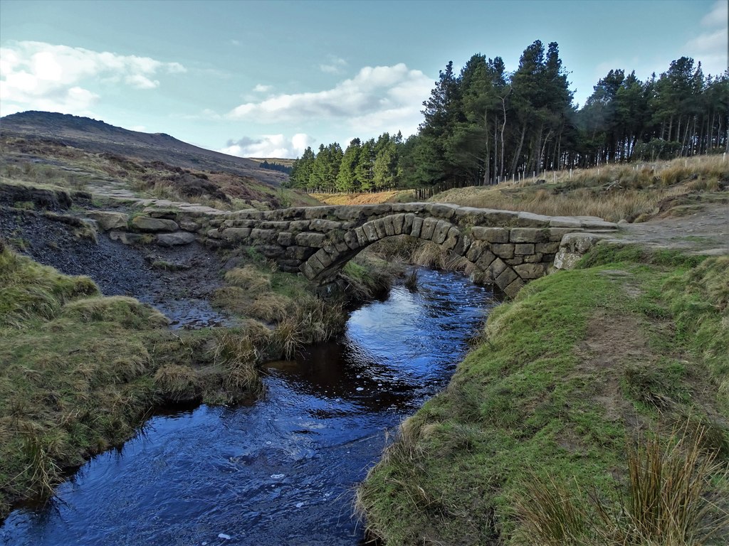
Figure: Packhorse Bridge under Burbage Edge. This packhorse route climbs steeply out of Hathersage and heads towards Sheffield. Packhorses were the main route for transporting goods across the Peak District. The high cost of transport is one driver of the ‘smith’ model, where there is a local skilled person responsible for assembling or creating goods (e.g. a blacksmith).

On Sunday mornings in Sheffield, I often used to run across Packhorse Bridge in Burbage valley. The bridge is part of an ancient network of trails crossing the Pennines that, before Turnpike roads arrived in the 18th century, was the main way in which goods were moved. Given that the moors around Sheffield were home to sand quarries, tin mines, lead mines and the villages in the Derwent valley were known for nail and pin manufacture, this wasn’t simply movement of agricultural goods, but it was the infrastructure for industrial transport.

The profession of leading the horses was known as a Jagger and leading out of the village of Hathersage is Jagger’s Lane, a trail that headed underneath Stanage Edge and into Sheffield.

The movement of goods from regions of supply to areas of demand is fundamental to our society. The physical infrastructure of supply chain has evolved a great deal over the last 300 years.

Cromford

[edit]

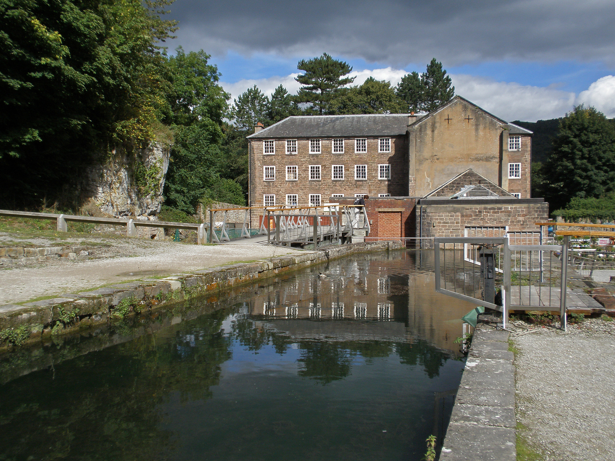
Figure: Richard Arkwright is regarded of the founder of the modern factory system. Factories exploit distribution networks to centralize production of goods. Arkwright located his factory in Cromford due to proximity to Nottingham Weavers (his market) and availability of water power from the tributaries of the Derwent river. When he first arrived there was almost no transportation network. Over the following 200 years The Cromford Canal (1790s), a Turnpike (now the A6, 1816-18) and the High Peak Railway (now closed, 1820s) were all constructed to improve transportation access as the factory blossomed.

Richard Arkwright is known as the father of the modern factory system. In 1771 he set up a Mill for spinning cotton yarn in the village of Cromford, in the Derwent Valley. The Derwent valley is relatively inaccessible. Raw cotton arrived in Liverpool from the US and India. It needed to be transported on packhorse across the bridleways of the Pennines. But Cromford was a good location due to proximity to Nottingham, where weavers where consuming the finished thread, and the availability of water power from small tributaries of the Derwent river for Arkwright’s water frames which automated the production of yarn from raw cotton.

By 1794 the Cromford Canal was opened to bring coal in to Cromford and give better transport to Nottingham. The construction of the canals was driven by the need to improve the transport infrastructure, facilitating the movement of goods across the UK. Canals, roads and railways were initially constructed by the economic need for moving goods. To improve supply chain.

The A6 now does pass through Cromford, but at the time he moved there there was merely a track. The High Peak Railway was opened in 1832, it is now converted to the High Peak Trail, but it remains the highest railway built in Britain.

Cooper (1991)

Containerization

[edit]

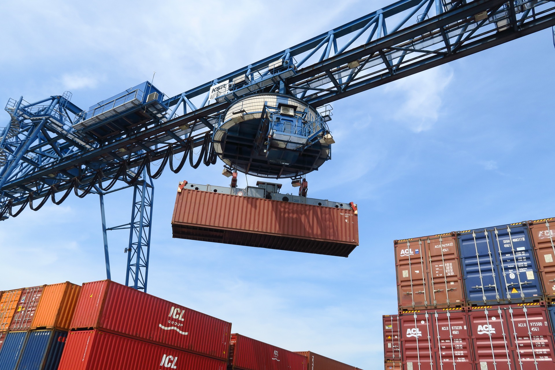
Figure: The container is one of the major drivers of globalization, and arguably the largest agent of social change in the last 100 years. It reduces the cost of transportation, significantly changing the appropriate topology of distribution networks. The container makes it possible to ship goods halfway around the world for cheaper than it costs to process those goods, leading to an extended distribution topology.

Containerization has had a dramatic effect on global economics, placing many people in the developing world at the end of the supply chain.

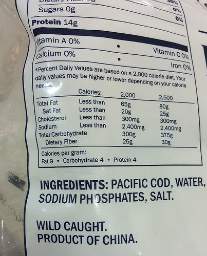
Figure: Wild Alaskan Cod, being solid in the Pacific Northwest, that is a product of China. It is cheaper to ship the deep frozen fish thousands of kilometers for processing than to process locally.

For example, you can buy Wild Alaskan Cod fished from Alaska, processed in China, sold in North America. This is driven by the low cost of transport for frozen cod vs the higher relative cost of cod processing in the US versus China. Similarly, Scottish prawns are also processed in China for sale in the UK.

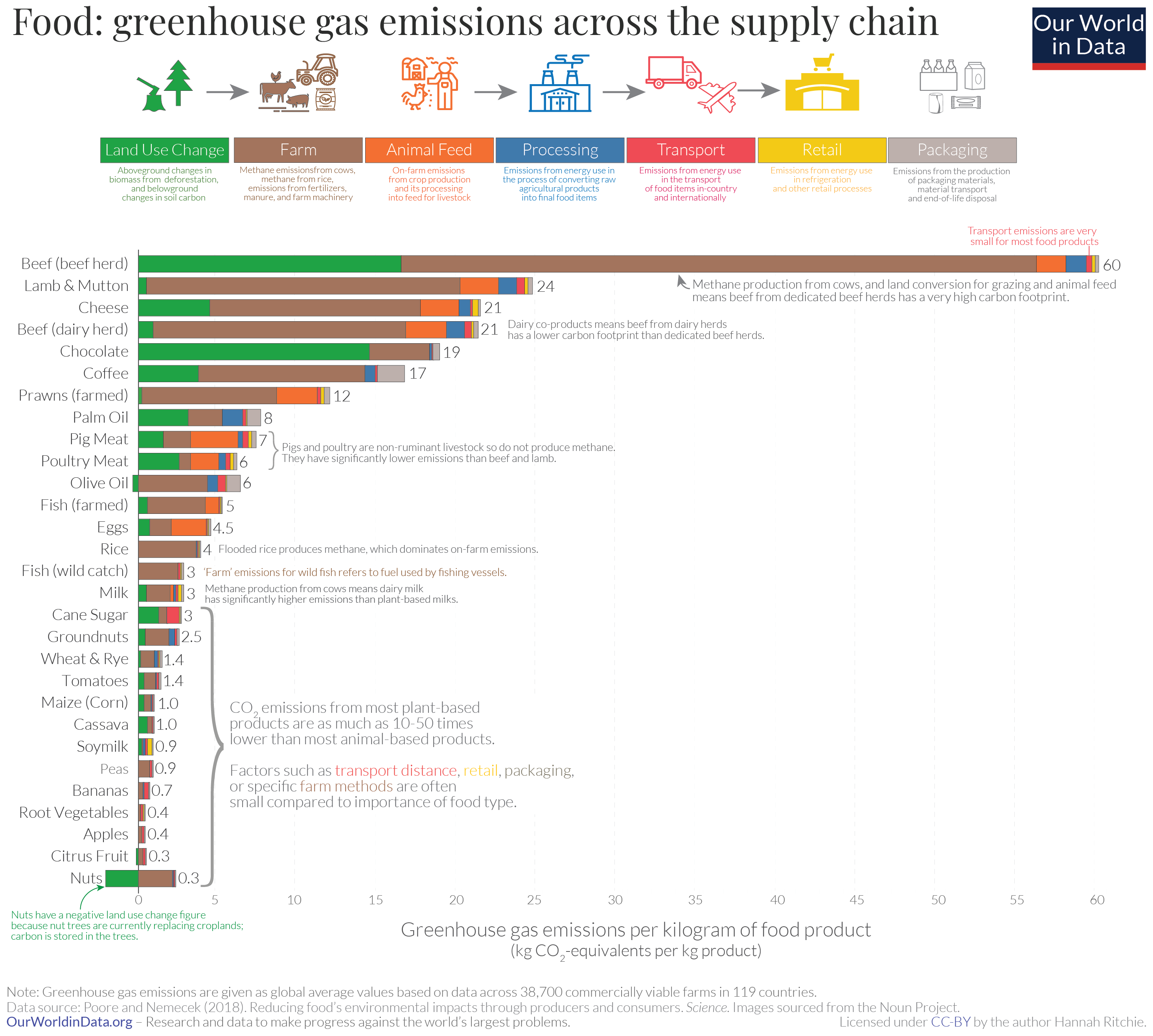
This effect on cost of transport vs cost of processing is the main driver of the topology of the modern supply chain and the associated effect of globalization. If transport is much cheaper than processing, then processing will tend to agglomerate in places where processing costs can be minimized.

Large scale global economic change has principally been driven by changes in the technology that drives supply chain.

Supply chain is a large-scale automated decision making network. Our aim is to make decisions not only based on our models of customer behavior (as observed through data), but also by accounting for the structure of our fulfilment center, and delivery network.

Many of the most important questions in supply chain take the form of counterfactuals. E.g. "What would happen if we opened a manufacturing facility in Cambridge?" A counter factual is a question that implies a mechanistic understanding of a system. It goes beyond simple smoothness assumptions or translation invariants. It requires a physical, or mechanistic understanding of the supply chain network. For this reason, the type of models we deploy in supply chain often involve simulations or more mechanistic understanding of the network.

In supply chain Machine Learning alone is not enough, we need to bridge between models that contain real mechanisms and models that are entirely data driven.

This is challenging, because as we introduce more mechanism to the models we use, it becomes harder to develop efficient algorithms to match those models to data.

Deploying Artificial Intelligence

[edit]

With the wide availability of new techniques, we are currently creating Artifical Intelligence through combination of machine learning algorithms to form machine learning systems.

This effect is amplified through the growth in sensorics, in particular the movement of cloud computing towards the customer. The barrier between cloud and device is blurring. This phenomenon is sometimes known as fog computing, or computing on the edge.

This presents major new challenges for machine learning systems design. We would like an internet of intelligence but currently our AI systems are fragile. A classical systems approach to design does not handle evolving environments well.

Data Science Africa

[edit]

Figure: Data Science Africa http://datascienceafrica.org is a ground up initiative for capacity building around data science, machine learning and artificial intelligence on the African continent.

Data Science Africa is a bottom up initiative for capacity building in data science, machine learning and artificial intelligence on the African continent.

As of 2019 there have been five workshops and five schools, located in Nyeri, Kenya (twice); Kampala, Uganda; Arusha, Tanzania; Abuja, Nigeria; Addis Ababa, Ethiopia and Accra, Ghana. The next event is scheduled for June 2020 in Kampala, Uganda.

The main notion is end-to-end data science. For example, going from data collection in the farmer’s field to decision making in the Ministry of Agriculture. Or going from malaria disease counts in health centers to medicine distribution.

The philosophy is laid out in (Lawrence 2015). The key idea is that the modern information infrastructure presents new solutions to old problems. Modes of development change because less capital investment is required to take advantage of this infrastructure. The philosophy is that local capacity building is the right way to leverage these challenges in addressing data science problems in the African context.

Data Science Africa is now a non-govermental organization registered in Kenya. The organising board of the meeting is entirely made up of scientists and academics based on the African continent.

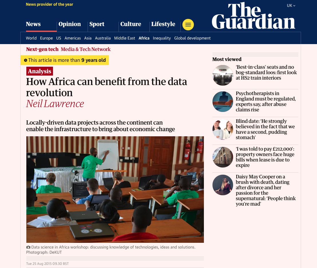
Figure: The lack of existing physical infrastructure on the African continent makes it a particularly interesting environment for deploying solutions based on the information infrastructure. The idea is explored more in this Guardian op-ed on Guardian article on How African can benefit from the data revolution.

Example: Prediction of Malaria Incidence in Uganda

[edit]

As an example of using Gaussian process models within the full pipeline from data to decsion, we’ll consider the prediction of Malaria incidence in Uganda. For the purposes of this study malaria reports come in two forms, HMIS reports from health centres and Sentinel data, which is curated by the WHO. There are limited sentinel sites and many HMIS sites.

The work is from Ricardo Andrade Pacheco’s PhD thesis, completed in collaboration with John Quinn and Martin Mubangizi (Andrade-Pacheco et al. 2014; Mubangizi et al. 2014). John and Martin were initally from the AI-DEV group from the University of Makerere in Kampala and more latterly they were based at UN Global Pulse in Kampala.

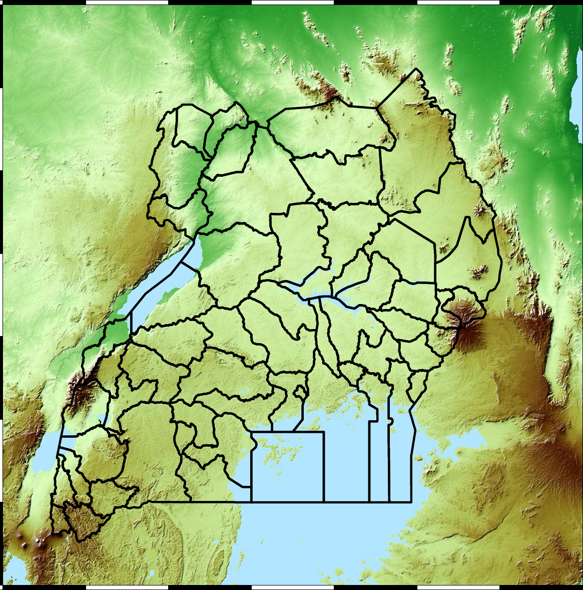
Malaria data is spatial data. Uganda is split into districts, and health reports can be found for each district. This suggests that models such as conditional random fields could be used for spatial modelling, but there are two complexities with this. First of all, occasionally districts split into two. Secondly, sentinel sites are a specific location within a district, such as Nagongera which is a sentinel site based in the Tororo district.

Figure: Ugandan districs. Data SRTM/NASA from https://dds.cr.usgs.gov/srtm/version2_1.

(Andrade-Pacheco et al. 2014; Mubangizi et al. 2014)

The common standard for collecting health data on the African continent is from the Health management information systems (HMIS). However, this data suffers from missing values (Gething et al. 2006) and diagnosis of diseases like typhoid and malaria may be confounded.

Figure: The Tororo district, where the sentinel site, Nagongera, is located.

World Health Organization Sentinel Surveillance systems are set up "when high-quality data are needed about a particular disease that cannot be obtained through a passive system". Several sentinel sites give accurate assessment of malaria disease levels in Uganda, including a site in Nagongera.

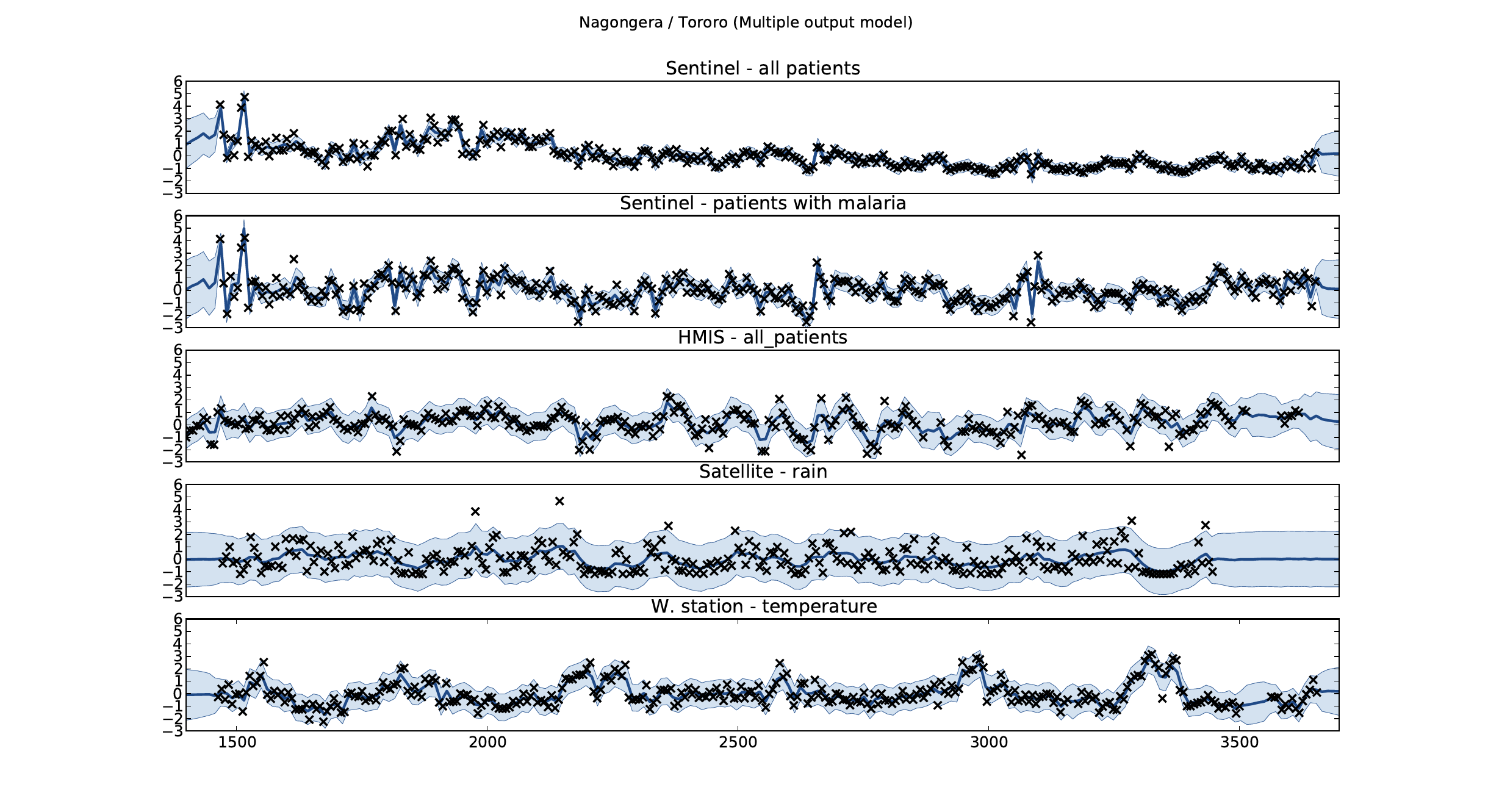
Figure: Sentinel and HMIS data along with rainfall and temperature for the Nagongera sentinel station in the Tororo district.

In collaboration with the AI Research Group at Makerere we chose to investigate whether Gaussian process models could be used to assimilate information from these two different sources of disease informaton. Further, we were interested in whether local information on rainfall and temperature could be used to improve malaria estimates.

The aim of the project was to use WHO Sentinel sites, alongside rainfall and temperature, to improve predictions from HMIS data of levels of malaria.

Figure: The Mubende District.

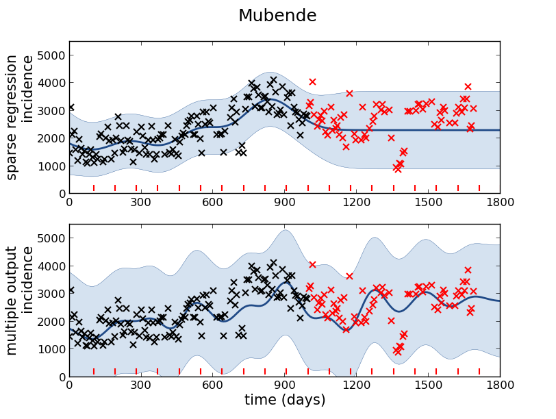
Figure: Prediction of malaria incidence in Mubende.

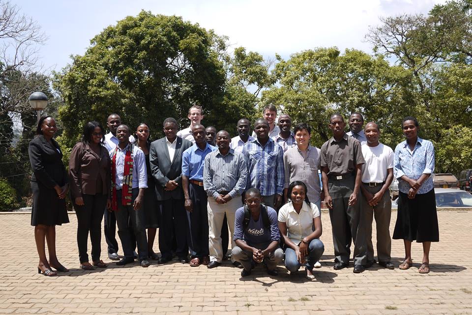
Figure: The project arose out of the Gaussian process summer school held at Makerere in Kampala in 2013. The school led, in turn, to the Data Science Africa initiative.

Early Warning Systems

Figure: The Kabarole district in Uganda.

Figure: Estimate of the current disease situation in the Kabarole district over time. Estimate is constructed with a Gaussian process with an additive covariance funciton.

Health monitoring system for the Kabarole district. Here we have fitted the reports with a Gaussian process with an additive covariance function. It has two components, one is a long time scale component (in red above) the other is a short time scale component (in blue).

Monitoring proceeds by considering two aspects of the curve. Is the blue line (the short term report signal) above the red (which represents the long term trend? If so we have higher than expected reports. If this is the case and the gradient is still positive (i.e. reports are going up) we encode this with a red color. If it is the case and the gradient of the blue line is negative (i.e. reports are going down) we encode this with an amber color. Conversely, if the blue line is below the red and decreasing, we color green. On the other hand if it is below red but increasing, we color yellow.

This gives us an early warning system for disease. Red is a bad situation getting worse, amber is bad, but improving. Green is good and getting better and yellow good but degrading.

Finally, there is a gray region which represents when the scale of the effect is small.

Figure: The map of Ugandan districts with an overview of the Malaria situation in each district.

These colors can now be observed directly on a spatial map of the districts to give an immediate impression of the current status of the disease across the country.

Conclusion

[edit]

Separation between machine learning and AI
Real world challenges such as matching supply to demand
Example of predicting disease via Gaussian processes

Thanks!

For more information on these subjects and more you might want to check the following resources.

References

Andrade-Pacheco, Ricardo, Martin Mubangizi, John Quinn, and Neil D. Lawrence. 2014. "Consistent Mapping of Government Malaria Records Across a Changing Territory Delimitation." Malaria Journal 13 (Suppl 1). https://doi.org/10.1186/1475-2875-13-S1-P5.

Cooper, Brian. 1991. Transformation of a Valley: Derbyshire Derwent. Scarthin Books.

Gething, Peter W., Abdisalan M. Noor, Priscilla W. Gikandi, Esther A. A. Ogara, Simon I. Hay, Mark S. Nixon, Robert W. Snow, and Peter M. Atkinson. 2006. "Improving Imperfect Data from Health Management Information Systems in Africa Using Space–Time Geostatistics." PLoS Medicine 3 (6). https://doi.org/10.1371/journal.pmed.0030271.

Lawrence, Neil D. 2015. "How Africa Can Benefit from the Data Revolution." The Guardian Media & Tech Network. https://www.theguardian.com/media-network/2015/aug/25/africa-benefit-data-science-information.

Mubangizi, Martin, Ricardo Andrade-Pacheco, Michael Thomas Smith, John Quinn, and Neil D. Lawrence. 2014. "Malaria Surveillance with Multiple Data Sources Using Gaussian Process Models." In 1st International Conference on the Use of Mobile ICT in Africa.

Wiener, Norbert. 1948. Cybernetics: Control and Communication in the Animal and the Machine. Cambridge, MA: MIT Press.