Abstract

Digital transformation has offered the promise of moving from a manual decision-making world to a world where decisions can be rational, data-driven and automated. The first step to digital transformation is mapping the world of atoms (material, customers, logistic networks) into the world of bits. But the real challenges may start once this is complete. In this talk we introduce the notion of ‘post digital transformation’: the challenges of doing business in a digital world.

Henry Ford’s Faster Horse

Figure: A 1925 Ford Model T built at Henry Ford’s Highland Park Plant in Dearborn, Michigan. This example now resides in Australia, owned by the founder of FordModelT.net. From https://commons.wikimedia.org/wiki/File:1925_Ford_Model_T_touring.jpg

It’s said that Henry Ford’s customers wanted a “a faster horse”. If Henry Ford was selling us artificial intelligence today, what would the customer call for, “a smarter human”? That’s certainly the picture of machine intelligence we find in science fiction narratives, but the reality of what we’ve developed is much more mundane.

Car engines produce prodigious power from petrol. Machine intelligences deliver decisions derived from data. In both cases the scale of consumption enables a speed of operation that is far beyond the capabilities of their natural counterparts. Unfettered energy consumption has consequences in the form of climate change. Does unbridled data consumption also have consequences for us?

If we devolve decision making to machines, we depend on those machines to accommodate our needs. If we don’t understand how those machines operate, we lose control over our destiny. Our mistake has been to see machine intelligence as a reflection of our intelligence. We cannot understand the smarter human without understanding the human. To understand the machine, we need to better understand ourselves.

Introduction

Setup

notutils

This small package is a helper package for various notebook utilities used below.

The software can be installed using

%pip install notutils

from the command prompt where you can access your python installation.

The code is also available on GitHub: https://github.com/lawrennd/notutils

Once notutils is installed, it can be imported in the usual manner.

import notutils

pods

In Sheffield we created a suite of software tools for ‘Open Data Science’. Open data science is an approach to sharing code, models and data that should make it easier for companies, health professionals and scientists to gain access to data science techniques.

You can also check this blog post on Open Data Science.

The software can be installed using

%pip install pods

from the command prompt where you can access your python installation.

The code is also available on GitHub: https://github.com/lawrennd/ods

Once pods is installed, it can be imported in the usual manner.

import pods

mlai

The mlai software is a suite of helper functions for teaching and demonstrating machine learning algorithms. It was first used in the Machine Learning and Adaptive Intelligence course in Sheffield in 2013.

The software can be installed using

%pip install mlai

from the command prompt where you can access your python installation.

The code is also available on GitHub: https://github.com/lawrennd/mlai

Once mlai is installed, it can be imported in the usual manner.

import mlai

The Gartner Hype Cycle

Figure: The Gartner Hype Cycle places technologies on a graph that relates to the expectations we have of a technology against its actual influence. Early hope for a new techology is often displaced by disillusionment due to the time it takes for a technology to be usefully deployed.

The Gartner Hype Cycle tries to assess where an idea is in terms of maturity and adoption. It splits the evolution of technology into a technological trigger, a peak of expectations followed by a trough of disillusionment and a final ascension into a useful technology. It looks rather like a classical control response to a final set point.

Cycle for ML Terms

Google Trends

%pip install pytrends

Figure: A Google trends search for ‘artificial intelligence’, ‘big data’, ‘data mining’, ‘deep learning’, ‘machine learning’ as different technological terms give us insight into their popularity over time.

Google trends gives us insight into the interest for different terms over time.

Examining Google trends search for ‘artificial intelligence’, ‘big data’, ‘data mining’, ‘deep learning’ and ‘machine learning’ we can see that ‘artificial intelligence’ may be entering a plateau of productivity, ‘big data’ is entering the trough of disillusionment, and ‘data mining’ seems to be deeply within the trough. On the other hand, ‘deep learning’ and ‘machine learning’ appear to be ascending to the peak of inflated expectations having experienced a technology trigger.

For deep learning that technology trigger was the ImageNet result of 2012 (Krizhevsky et al., n.d.). This step change in performance on object detection in images was achieved through convolutional neural networks, popularly known as ‘deep learning’.

What is Machine Learning?

What is machine learning? At its most basic level machine learning is a combination of

\[\text{data} + \text{model} \stackrel{\text{compute}}{\rightarrow} \text{prediction}\]

where data is our observations. They can be actively or passively acquired (meta-data). The model contains our assumptions, based on previous experience. That experience can be other data, it can come from transfer learning, or it can merely be our beliefs about the regularities of the universe. In humans our models include our inductive biases. The prediction is an action to be taken or a categorization or a quality score. The reason that machine learning has become a mainstay of artificial intelligence is the importance of predictions in artificial intelligence. The data and the model are combined through computation.

In practice we normally perform machine learning using two functions. To combine data with a model we typically make use of:

a prediction function it is used to make the predictions. It includes our beliefs about the regularities of the universe, our assumptions about how the world works, e.g., smoothness, spatial similarities, temporal similarities.

an objective function it defines the ‘cost’ of misprediction. Typically, it includes knowledge about the world’s generating processes (probabilistic objectives) or the costs we pay for mispredictions (empirical risk minimization).

The combination of data and model through the prediction function and the objective function leads to a learning algorithm. The class of prediction functions and objective functions we can make use of is restricted by the algorithms they lead to. If the prediction function or the objective function are too complex, then it can be difficult to find an appropriate learning algorithm. Much of the academic field of machine learning is the quest for new learning algorithms that allow us to bring different types of models and data together.

A useful reference for state of the art in machine learning is the UK Royal Society Report, Machine Learning: Power and Promise of Computers that Learn by Example.

You can also check my post blog post on What is Machine Learning?.

Artificial Intelligence and Data Science

Artificial intelligence has the objective of endowing computers with human-like intelligent capabilities. For example, understanding an image (computer vision) or the contents of some speech (speech recognition), the meaning of a sentence (natural language processing) or the translation of a sentence (machine translation).

Supervised Learning for AI

The machine learning approach to artificial intelligence is to collect and annotate a large data set from humans. The problem is characterized by input data (e.g. a particular image) and a label (e.g. is there a car in the image yes/no). The machine learning algorithm fits a mathematical function (I call this the prediction function) to map from the input image to the label. The parameters of the prediction function are set by minimizing an error between the function’s predictions and the true data. This mathematical function that encapsulates this error is known as the objective function.

This approach to machine learning is known as supervised learning. Various approaches to supervised learning use different prediction functions, objective functions or different optimization algorithms to fit them.

For example, deep learning makes use of neural networks to form the predictions. A neural network is a particular type of mathematical function that allows the algorithm designer to introduce invariances into the function.

An invariance is an important way of including prior understanding in a machine learning model. For example, in an image, a car is still a car regardless of whether it’s in the upper left or lower right corner of the image. This is known as translation invariance. A neural network encodes translation invariance in convolutional layers. Convolutional neural networks are widely used in image recognition tasks.

An alternative structure is known as a recurrent neural network (RNN). RNNs neural networks encode temporal structure. They use auto regressive connections in their hidden layers, they can be seen as time series models which have non-linear auto-regressive basis functions. They are widely used in speech recognition and machine translation.

Machine learning has been deployed in Speech Recognition (e.g. Alexa, deep neural networks, convolutional neural networks for speech recognition), in computer vision (e.g. Amazon Go, convolutional neural networks for person recognition and pose detection).

The field of data science is related to AI, but philosophically different. It arises because we are increasingly creating large amounts of data through happenstance rather than active collection. In the modern era data is laid down by almost all our activities. The objective of data science is to extract insights from this data.

Classically, in the field of statistics, data analysis proceeds by assuming that the question (or scientific hypothesis) comes before the data is created. E.g., if I want to determine the effectiveness of a particular drug, I perform a design for my data collection. I use foundational approaches such as randomization to account for confounders. This made a lot of sense in an era where data had to be actively collected. The reduction in cost of data collection and storage now means that many data sets are available which weren’t collected with a particular question in mind. This is a challenge because bias in the way data was acquired can corrupt the insights we derive. We can perform randomized control trials (or A/B tests) to verify our conclusions, but the opportunity is to use data science techniques to better guide our question selection or even answer a question without the expense of a full randomized control trial (referred to as A/B testing in modern internet parlance).

Intellectual Debt

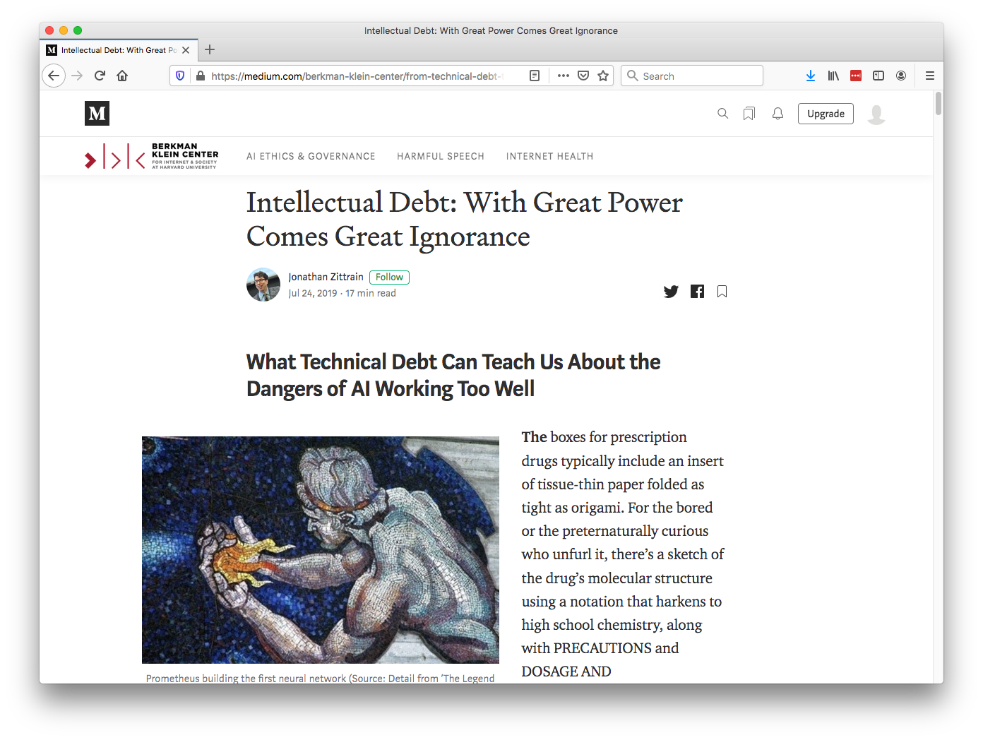
Figure: Jonathan Zittrain’s term to describe the challenges of explanation that come with AI is Intellectual Debt.

Information and Embodiment

Claude Shannon

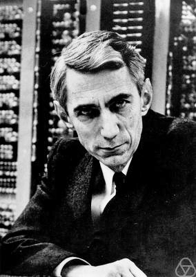
Figure: Claude Shannon (1916-2001)

bits/min	billions	2,000
billion calculations/s	~100	a billion
embodiment	20 minutes	5 billion years

Figure: Embodiment factors are the ratio between our ability to compute and our ability to communicate. Relative to the machine we are also locked in. In the table we represent embodiment as the length of time it would take to communicate one second’s worth of computation. For computers it is a matter of minutes, but for a human, it is a matter of thousands of millions of years.

A Six Word Novel

Figure: Consider the six-word novel, apocryphally credited to Ernest Hemingway, “For sale: baby shoes, never worn”. To understand what that means to a human, you need a great deal of additional context. Context that is not directly accessible to a machine that has not got both the evolved and contextual understanding of our own condition to realize both the implication of the advert and what that implication means emotionally to the previous owner.

But this is a very different kind of intelligence than ours. A computer cannot understand the depth of the Ernest Hemingway’s apocryphal six-word novel: “For Sale, Baby Shoes, Never worn”, because it isn’t equipped with that ability to model the complexity of humanity that underlies that statement.

Bandwidth Constrained Conversations

Figure: Conversation relies on internal models of other individuals.

Figure: Misunderstanding of context and who we are talking to leads to arguments.

Embodiment factors imply that, in our communication between humans, what is not said is, perhaps, more important than what is said. To communicate with each other we need to have a model of who each of us are.

To aid this, in society, we are required to perform roles. Whether as a parent, a teacher, an employee or a boss. Each of these roles requires that we conform to certain standards of behaviour to facilitate communication between ourselves.

Control of self is vitally important to these communications.

The high availability of data available to humans undermines human-to-human communication channels by providing new routes to undermining our control of self.

The consequences between this mismatch of power and delivery are to be seen all around us. Because, just as driving an F1 car with bicycle wheels would be a fine art, so is the process of communication between humans.

If I have a thought and I wish to communicate it, I first need to have a model of what you think. I should think before I speak. When I speak, you may react. You have a model of who I am and what I was trying to say, and why I chose to say what I said. Now we begin this dance, where we are each trying to better understand each other and what we are saying. When it works, it is beautiful, but when mis-deployed, just like a badly driven F1 car, there is a horrible crash, an argument.

Evolved Relationship with Information

The high bandwidth of computers has resulted in a close relationship between the computer and data. Large amounts of information can flow between the two. The degree to which the computer is mediating our relationship with data means that we should consider it an intermediary.

Originally our low bandwidth relationship with data was affected by two characteristics. Firstly, our tendency to over-interpret driven by our need to extract as much knowledge from our low bandwidth information channel as possible. Secondly, by our improved understanding of the domain of mathematical statistics and how our cognitive biases can mislead us.

With this new set up there is a potential for assimilating far more information via the computer, but the computer can present this to us in various ways. If its motives are not aligned with ours then it can misrepresent the information. This needn’t be nefarious it can be simply because of the computer pursuing a different objective from us. For example, if the computer is aiming to maximize our interaction time that may be a different objective from ours which may be to summarize information in a representative manner in the shortest possible length of time.

For example, for me, it was a common experience to pick up my telephone with the intention of checking when my next appointment was, but to soon find myself distracted by another application on the phone and end up reading something on the internet. By the time I’d finished reading, I would often have forgotten the reason I picked up my phone in the first place.

There are great benefits to be had from the huge amount of information we can unlock from this evolved relationship between us and data. In biology, large scale data sharing has been driven by a revolution in genomic, transcriptomic and epigenomic measurement. The improved inferences that can be drawn through summarizing data by computer have fundamentally changed the nature of biological science, now this phenomenon is also influencing us in our daily lives as data measured by happenstance is increasingly used to characterize us.

Better mediation of this flow requires a better understanding of human-computer interaction. This in turn involves understanding our own intelligence better, what its cognitive biases are and how these might mislead us.

For further thoughts see Guardian article on marketing in the internet era from 2015.

You can also check my blog post on System Zero. This was also written in 2015.

New Flow of Information

Classically the field of statistics focused on mediating the relationship between the machine and the human. Our limited bandwidth of communication means we tend to over-interpret the limited information that we are given, in the extreme we assign motives and desires to inanimate objects (a process known as anthropomorphizing). Much of mathematical statistics was developed to help temper this tendency and understand when we are valid in drawing conclusions from data.

Figure: The trinity of human, data, and computer, and highlights the modern phenomenon. The communication channel between computer and data now has an extremely high bandwidth. The channel between human and computer and the channel between data and human is narrow. New direction of information flow, information is reaching us mediated by the computer. The focus on classical statistics reflected the importance of the direct communication between human and data. The modern challenges of data science emerge when that relationship is being mediated by the machine.

Data science brings new challenges. In particular, there is a very large bandwidth connection between the machine and data. This means that our relationship with data is now commonly being mediated by the machine. Whether this is in the acquisition of new data, which now happens by happenstance rather than with purpose, or the interpretation of that data where we are increasingly relying on machines to summarize what the data contains. This is leading to the emerging field of data science, which must not only deal with the same challenges that mathematical statistics faced in tempering our tendency to over interpret data but must also deal with the possibility that the machine has either inadvertently or maliciously misrepresented the underlying data.

Revolution

Arguably the information revolution we are experiencing is unprecedented in history. But changes in the way we share information have a long history. Over 5,000 years ago in the city of Uruk, on the banks of the Euphrates, communities which relied on the water to irrigate their corps developed an approach to recording transactions in clay. Eventually the system of recording system became sophisticated enough that their oral histories could be recorded in the form of the first epic: Gilgamesh.

Figure: Chicago Stone, side 2, recording sale of a number of fields, probably from Isin, Early Dynastic Period, c. 2600 BC, black basalt

It was initially develoepd for people as a recordd of who owed what to whom, expanding individuals’ capacity to remember. But over a five hundred year period writing evolved to become a tool for literature as well. More pithily put, writing was invented by accountants not poets (see e.g. this piece by Tim Harford).

In some respects today’s revolution is different, because it involves also the creation of stories as well as their curation. But in some fundamental ways we can see what we have produced as another tool for us in the information revolution.

The Future of Professions

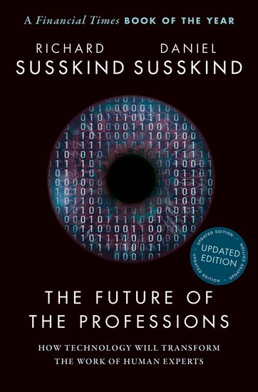
Figure: The Future of Professions (Susskind and Susskind, 2015) is a 2015 book focussed on how the next wave of technology revolution is going to effect the professions.

And this is very likely true, but in practice we know that even if the disruption is being felt initially by the professional classes, those groups tend to be protected by their ability to adapt, which is correlated with higher education.

Whether this remains true this time is another question. I’m particularly struck by the “convergent evolution” of ChatGPT. The model is trained by reinforcement learning with feedback provided by people. ChatGPT’s answers are highly plausible, make use of sophisticated language in an intelligent sounding way and are often incorrect. I’m struck by the similarity to fresh Oxbridge graduates. I wonder if this is also an example of convergent evolution.

Coin Pusher

Disruption of society is like a coin pusher, it’s those who are already on the edge who are most likely to be effected by disruption.

Figure: A coin pusher is a game where coins are dropped into th etop of the machine, and they disrupt those on the existing steps. With any coin drop, many coins move, but it is those on the edge, who are often only indirectly effected, but also most traumatically effected by the change.

One danger of the current hype around ChatGPT is that we are overly focussing on the fact that it seems to have significant effect on professional jobs, people are naturally asking the question “what does it do for my role?”. No doubt, there will be disruption, but the coin pusher hypothesis suggests that that disruption will likely involve movement on the same step. However it is those on the edge already, who are often not working directly in the information economy, who often have less of a voice in the policy conversation who are likely to be most disrupted.

Royal Society Report

Figure: The Royal Society report on Machine Learning was released on 25th April 2017

Public Research

Figure: The Royal Society comissioned public research from Mori as part of the machine learning review.

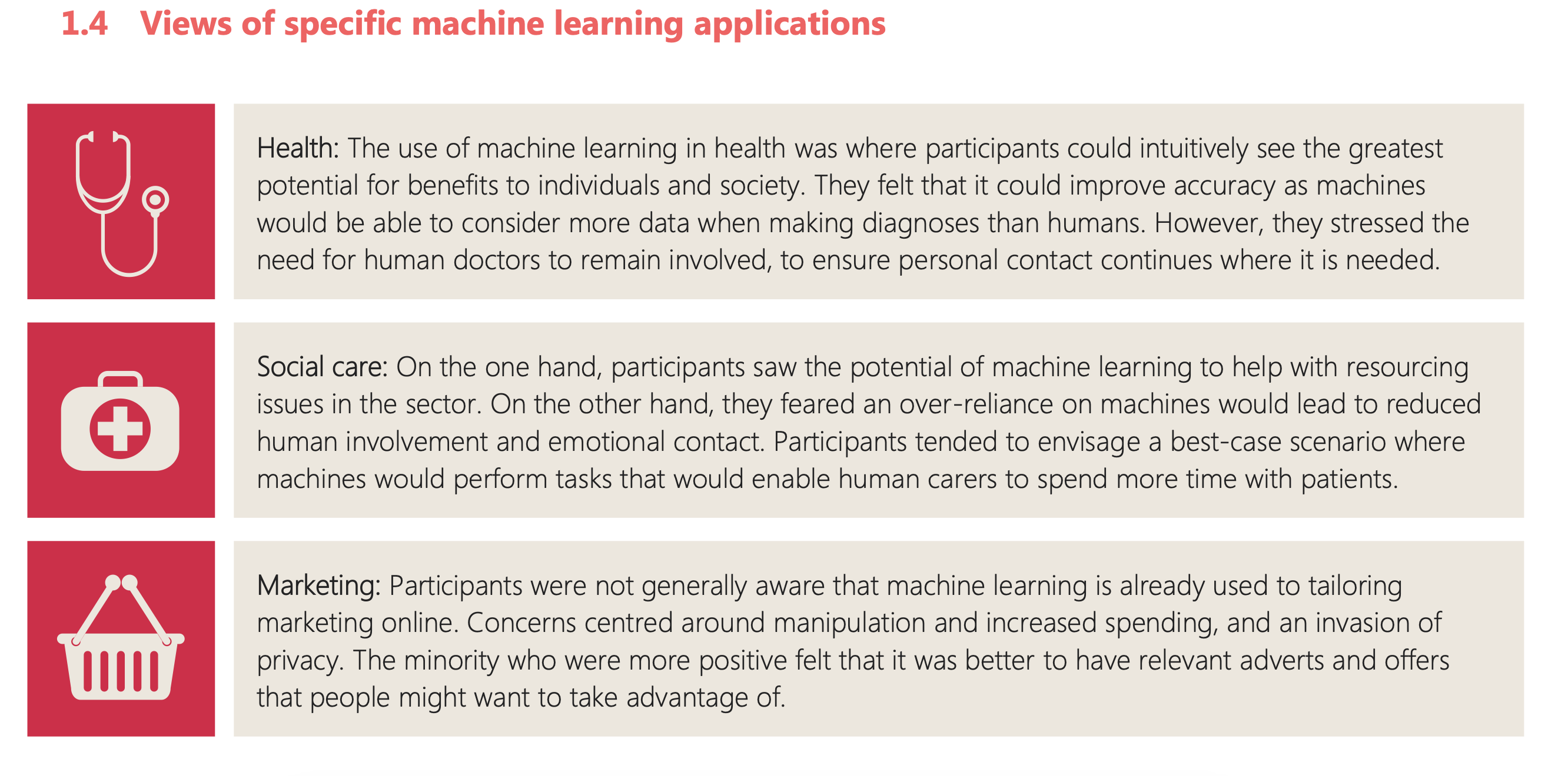
Figure: One of the questions focussed on machine learning applications.

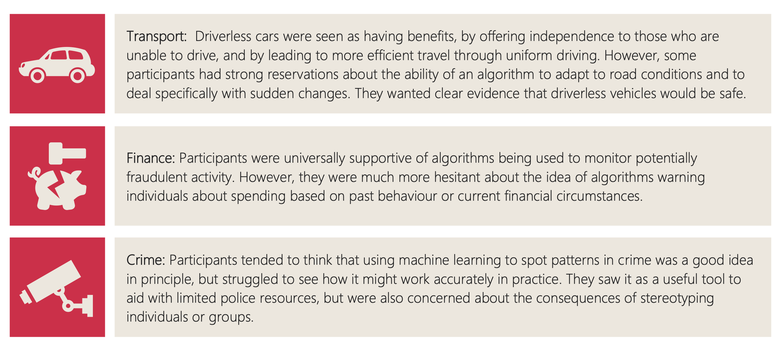
Figure: The public were broadly supportive of a range of application areas.

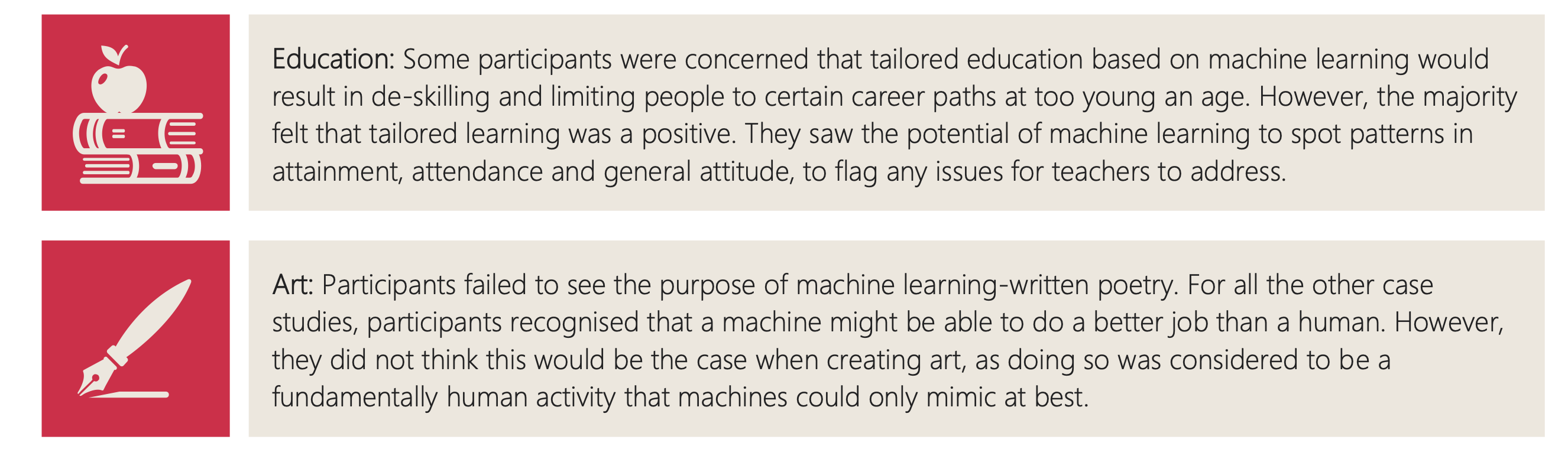
Figure: But they failed to see the point in AI’s that could produce poetry.

Mercutio

It’s ironic that despite the public focus on transport, health, cities, crime and their confusion as to why we might want AI to do art, one area where significant progress has been made is on AIs that can create literature.

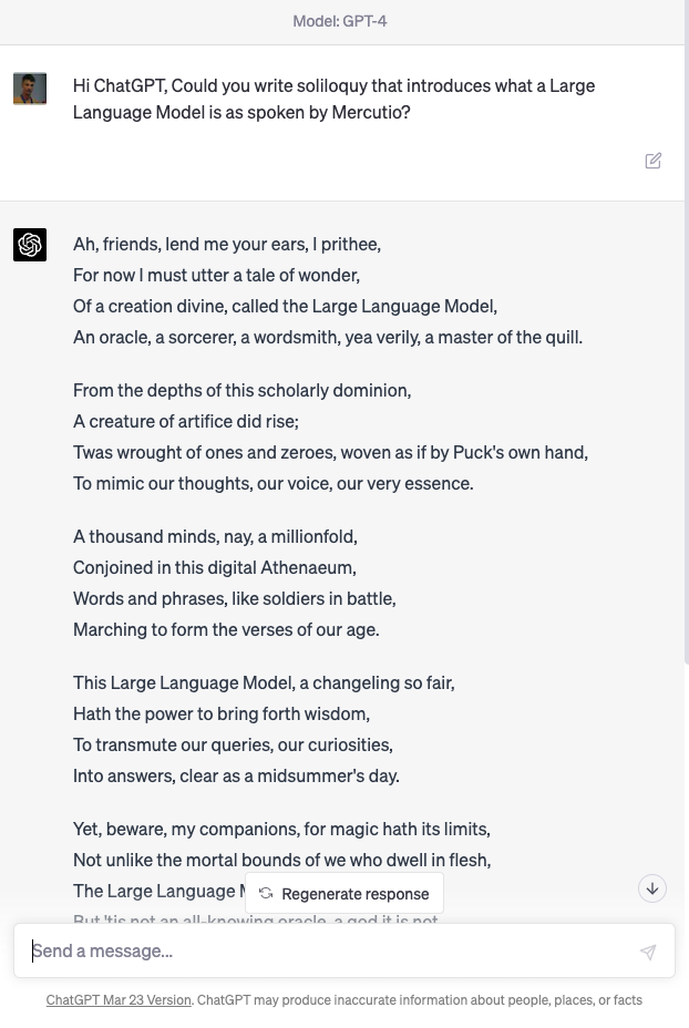
Figure: Despite the public’s desire to see challenges in health, finance, transport, crime solved by machine learning and their skepticism around poetry, one of the problems we have solved seems to be poetry.

User: Hi ChatGPT, Could you write soliloquy that introduces what a Large Language Model is as spoken by Mercutio?

Machine: Ah, friends, lend me your ears, I prithee, For now I must utter a tale of wonder, Of a creation divine, called the Large Language Model, An oracle, a sorcerer, a wordsmith, yea verily, a master of the quill.

From the depths of this scholarly dominion, A creature of artifice did rise; Twas wrought of ones and zeroes, woven as if by Puck’s own hand, To mimic our thoughts, our voice, our very essence.

A thousand minds, nay, a millionfold, Conjoined in this digital Athenaeum, Words and phrases, like soldiers in battle, Marching to form the verses of our age.

This Large Language Model, a changeling so fair, Hath the power to bring forth wisdom, To transmute our queries, our curiosities, Into answers, clear as a midsummer’s day.

Yet, beware, my companions, for magic hath its limits, Not unlike the mortal bounds of we who dwell in flesh, The Large Language Model hath its strengths, But ’tis not an all-knowing oracle, a god it is not.

As Mercutio, your humble servant, doth stand before thee, I marvel at the art and science that hath brought forth this wondrous creation, This Large Language Model, a testament to man’s yearning, To comprehend the world and make meaning of the great tapestry of existence.

In faith, dear friends, let us embrace the magic and beauty of this digital bard, And mayhaps, by its grace, we shall glean some wisdom, As we wander together, hand in hand, Through this boundless realm of knowledge and wonder.

ChatGPT transcript, 14th April 2023.

Weather

So what’s going on here? One analogy I like to use is with weather forecasting. Historically, before the use of computer driven weather forecasting, we used a process of interpolation to measure the pressure.

Figure: Forecast from UK Met Office on 5th June 1944. (detail from https://www.metoffice.gov.uk/research/library-and-archive/archive-hidden-treasures/d-day)

This was problematic for German forces in the Second World War because they had no ability to predict the weather when it was coming in from across the UK. Conversely, the UK had a number of weather stations in the UK, and some information (perhaps from spies or Enigma decrypts) about weather on the mainland.

Figure: Forecast from Deutscher Wetterdienst on 5th June 1944. (detail from https://www.metoffice.gov.uk/research/library-and-archive/archive-hidden-treasures/d-day). Note the lack of measurements within the UK. THis is the direction that weather was coming from so the locaiton of weather fronts (and associated storms) was harder for the Deutscher Wetterdienst to predict than the Met Office.

This meant that more accurate forecasts were possible for D-Day for the Allies than for the defending forces. As a result, on the morning that Eisenhower invated, Rommel was back in Germany attending his wife’s 50th birthday party.

\(p\)-Fairness and \(n\)-Fairness

Figure: We seem to have two different aspects to fairness, which in practice can be in tension.

We’ve outlined \(n\)-fairness and \(p\)-fairness. By \(n\)-fairness we mean the sort of considerations that are associated with substantive equality of opportunity vs formal equality of opportunity. Formal equality of community is related to \(p\)-fairness. This is sometimes called procedural fairness and we might think of it as a performative form of fairness. It’s about clarity of rules, for example as applied in sport. \(n\)-Fairness is more nuanced. It’s a reflection of society’s normative judgment about how individuals may have been disadvantaged, e.g. due to their upbringing.

The important point here is that these forms of fairness are in tension. Good procedural fairness needs to be clear and understandable. It should be clear to everyone what the rules are, they shouldn’t be obscured by jargon or overly subtle concepts. \(p\)-Fairness should not be easily undermined by adversaries, it should be difficult to “cheat” good \(p\)-fairness. However, \(n\)-fairness requires nuance, understanding of the human condition, where we came from and how different individuals in our society have been advantaged or disadvantaged in their upbringing and their access to opportunity.

Pure \(n\)-fairness and pure \(p\)-fairness both have the feeling of dystopias. In practice, any decision making system needs to balance the two. The correct point of operation will depend on the context of the decision. Consider fair rules of a game of football, against fair distribution of social benefit. It is unlikely that there is ever an objectively correct balance between the two for any given context. Different individuals will favour \(p\) vs \(n\) according to their personal values.

Given the tension between the two forms of fairness, with \(p\) fairness requiring simple rules that are understandable by all, and \(n\) fairness requiring nuance and subtlety, how do we resolve this tension in practice?

Normally in human systems, significant decisions involve trained professionals. For example, judges, or accountants or doctors.

Training a professional involves lifting their “reflexive” response to a situation with “reflective” thinking about the consequences of their decision that rely not just on the professional’s expertise, but also their knowledge of what it is to be a human.

This marvellous resolution exploits the fact that while humans are increadibly complicated nuanced entities, other humans have an intuitive ability to understand their motivations and values. So the human is a complex entity that seems simple to other humans.

A Question of Trust

In Baroness Onora O’Neill’s Reeith Lectures from 2002, she raises the challenge of trust. There are many aspects to her arcuments, but one of the key points she makes is that we cannot trust without the notion of duty. O’Neill is bemoaning the substitution of duty with process. The idea is that processes and transparency are supposed to hold us to account by measuring outcomes. But these processes themselves overwhelm decision makers and undermine their professional duty to deliver the right outcome.

Figure: A Question of Trust by Onora O’Neil which examines the nature of trust and its role in society.

Again Univesities are to treat each applicant fairly on the basis of ability and promise, but they are supposed also to admit a socially more representative intake.

There’s no guarantee that the process meets the target.

Onora O’Neill A Question of Trust: Called to Account Reith Lectures 2002 O’Neill (2002)]

O’Neill is speaking in 2002, in the early days of the internet and before social media. Much of her thoughts are even more relevant for today than they were when she spoke. This is because the increased availability of information and machine driven decision-making makes the mistaken premise, that process is an adequate substitute for duty, more apparently plausible. But this undermines what O’Neill calls “intelligent accountability”, which is not accounting by the numbers, but through professional education and institutional safeguards.

Complexity in Action

As an exercise in understanding complexity, watch the following video. You will see the basketball being bounced around, and the players moving. Your job is to count the passes of those dressed in white and ignore those of the individuals dressed in black.

Figure: Daniel Simon’s famous illusion “monkey business”. Focus on the movement of the ball distracts the viewer from seeing other aspects of the image.

In a classic study Simons and Chabris (1999) ask subjects to count the number of passes of the basketball between players on the team wearing white shirts. Fifty percent of the time, these subjects don’t notice the gorilla moving across the scene.

The phenomenon of inattentional blindness is well known, e.g in their paper Simons and Charbris quote the Hungarian neurologist, Rezsö Bálint,

It is a well-known phenomenon that we do not notice anything happening in our surroundings while being absorbed in the inspection of something; focusing our attention on a certain object may happen to such an extent that we cannot perceive other objects placed in the peripheral parts of our visual field, although the light rays they emit arrive completely at the visual sphere of the cerebral cortex.

Rezsö Bálint 1907 (translated in Husain and Stein 1988, page 91)

When we combine the complexity of the world with our relatively low bandwidth for information, problems can arise. Our focus on what we perceive to be the most important problem can cause us to miss other (potentially vital) contextual information.

This phenomenon is known as selective attention or ‘inattentional blindness’.

Figure: For a longer talk on inattentional bias from Daniel Simons see this video.

Data Selective Attention Bias

We are going to see how inattention biases can play out in data analysis by going through a simple example. The analysis involves body mass index and activity information.

BMI Steps Data

The BMI Steps example is taken from Yanai and Lercher (2020). We are given a data set of body-mass index measurements against step counts. For convenience we have packaged the data so that it can be easily downloaded.

import pods

data = pods.datasets.bmi_steps()
X = data['X'] 
y = data['Y']

It is good practice to give our variables interpretable names so that the analysis may be clearly understood by others. Here the steps count is the first dimension of the covariate, the bmi is the second dimension and the gender is stored in y with 1 for female and 0 for male.

steps = X[:, 0]
bmi = X[:, 1]
gender = y[:, 0]

We can check the mean steps and the mean of the BMI.

print('Steps mean is {mean}.'.format(mean=steps.mean()))

print('BMI mean is {mean}.'.format(mean=bmi.mean()))

BMI Steps Data Analysis

We can also separate out the means from the male and female populations. In python this can be done by setting male and female indices as follows.

male_ind = (gender==0)
female_ind = (gender==1)

And now we can extract the variables for the two populations.

male_steps = steps[male_ind]
male_bmi = bmi[male_ind]

And as before we compute the mean.

print('Male steps mean is {mean}.'.format(mean=male_steps.mean()))

print('Male BMI mean is {mean}.'.format(mean=male_bmi.mean()))

Similarly, we can get the same result for the female portion of the populaton.

female_steps = steps[female_ind]
female_bmi = bmi[female_ind]

print('Female steps mean is {mean}.'.format(mean=female_steps.mean()))

print('Female BMI mean is {mean}.'.format(mean=female_bmi.mean()))

Interesting, the female BMI average is slightly higher than the male BMI average. The number of steps in the male group is higher than that in the female group. Perhaps the steps and the BMI are anti-correlated. The more steps, the lower the BMI.

Python provides a statistics package. We’ll import this in python so that we can try and understand the correlation between the steps and the BMI.

from scipy.stats import pearsonr

corr, _ = pearsonr(steps, bmi)
print("Pearson's overall correlation: {corr}".format(corr=corr))

male_corr, _ = pearsonr(male_steps, male_bmi)
print("Pearson's correlation for males: {corr}".format(corr=male_corr))

female_corr, _ = pearsonr(female_steps, female_bmi)
print("Pearson's correlation for females: {corr}".format(corr=female_corr))

A Hypothesis as a Liability

This analysis is from an article titled “A Hypothesis as a Liability” (Yanai and Lercher, 2020), they start their article with the following quite from Herman Hesse.

“ ‘When someone seeks,’ said Siddhartha, ‘then it easily happens that his eyes see only the thing that he seeks, and he is able to find nothing, to take in nothing. […] Seeking means: having a goal. But finding means: being free, being open, having no goal.’ ”

Hermann Hesse

Their idea is that having a hypothesis can constrain our thinking. However, in answer to their paper Felin et al. (2021) argue that some form of hypothesis is always necessary, suggesting that a hypothesis can be a liability

My view is captured in the introductory chapter to an edited volume on computational systems biology that I worked on with Mark Girolami, Magnus Rattray and Guido Sanguinetti.

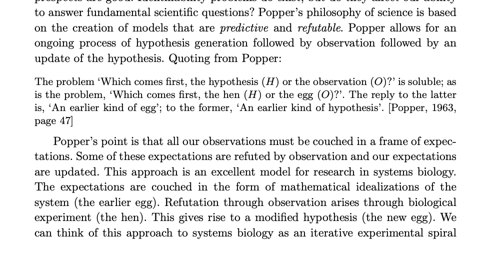
Figure: Quote from Lawrence (2010) highlighting the importance of interaction between data and hypothesis.

Popper nicely captures the interaction between hypothesis and data by relating it to the chicken and the egg. The important thing is that these two co-evolve.

Number Theatre

Unfortunately, we don’t always have time to wait for this process to converge to an answer we can all rely on before a decision is required.

Not only can we be misled by data before a decision is made, but sometimes we can be misled by data to justify the making of a decision. David Spiegelhalter refers to the phenomenon of “Number Theatre” in a conversation with Andrew Marr from May 2020 on the presentation of data.

Figure: Professor Sir David Spiegelhalter on Andrew Marr on 10th May 2020 speaking about some of the challengers around data, data presentation, and decision making in a pandemic. David mentions number theatre at 9 minutes 10 seconds.

Data Theatre

Data Theatre exploits data inattention bias to present a particular view on events that may misrepresents through selective presentation. Statisticians are one of the few groups that are trained with a sufficient degree of data skepticism. But it can also be combatted through ensuring there are domain experts present, and that they can speak freely.

Figure: The phenomenon of number theatre or data theatre was described by David Spiegelhalter and is nicely summarized by Martin Robbins in this sub-stack article https://martinrobbins.substack.com/p/data-theatre-why-the-digital-dashboards.

The Art of Statistics

The statistician’s craft is based on humility in front of data and developing the appropriate skeptical thinking around conclusions from data. The best book I’ve seen for developing that sense is Sir David Spiegelhalter’s Art of Statistics.

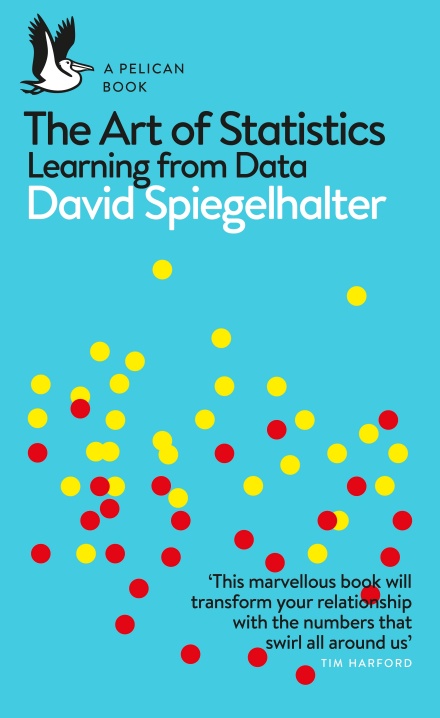
Figure: The Art of Statistics by David Spiegelhalter is an excellent read on the pitfalls of data interpretation.

David’s book (Spiegelhalter, 2019) brings important examples from statistics to life in an intelligent and entertaining way. It is highly readable and gives an opportunity to fast-track towards the important skill of data-skepticism that is the mark of a professional statistician.

Conclusion

See the Gorilla don’t be the Gorilla.

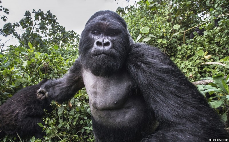
Figure: A famous quote from Mike Tyson before his fight with Evander Holyfield: “Everyone has a plan until they get punched in the mouth”. Don’t let the gorilla punch you in the mouth. See the gorilla, but don’t be the gorilla. Photo credit: https://www.catersnews.com/stories/animals/go-ape-unlucky-photographer-gets-punched-by-lairy-gorilla-drunk-from-eating-bamboo-shoots/

AI@Cam

AI@Cam is a new flagship University mission that seeks to address these challenges. It recognises that development of safe and effective AI-enabled innovations requires this mix of expertise from across research domains, businesses, policy-makers, civill society, and from affected communities. AI@Cam is setting out a vision for AI-enabled innovation that benefits science, citizens and society.

This vision will be achieved through leveraging the University’s vibrant interdisciplinary research community. AI@Cam will form partnerships between researchers, practitioners, and affected communities that embed equity and inclusion. It will develop new platforms for innovation and knowledge transfer. It will deliver innovative interdisciplinary teaching and learning for students, researchers, and professionals. It will build strong connections between the University and national AI priorities.

The University operates as both an engine of AI-enabled innovation and steward of those innovations.

AI is not a universal remedy. It is a set of tools, techniques and practices that correctly deployed can be leveraged to deliver societal benefit and mitigate social harm.

In that sense AI@Cam’s mission is close in spirit to that of Panacea’s elder sister Hygeia. It is focussed on building and maintaining the hygiene of a robust and equitable AI research ecosystem.

Figure: AI@Cam is a Flagship Programme that supports AI research across the University.

Finally, we are working across the University to empower the diversity ofexpertise and capability we have to focus on these broad societal problems. We will recently launched AI@Cam with a vision document that outlines these challenges for the University.

The initiative was funded in November 2022 where a £5M investment from the University was secured.

Progress so far:

• Developing the vision
  • Engaged over 100 members of the University community across 30 departments/institutes, start-ups, and large businesses.
  • Supported 6 new funding bids

Further Reading

• Chapter 8 of Lawrence (2024)

Thanks!

For more information on these subjects and more you might want to check the following resources.

• twitter: @lawrennd
• podcast: The Talking Machines
• newspaper: Guardian Profile Page
• blog: http://inverseprobability.com