Abstract

Digital transformation has offered the promise of moving from a manual decision-making world to a world where decisions can be rational, data-driven and automated. The first step to digital transformation is mapping the world of atoms (material, customers, logistic networks) into the world of bits. But the real challenges may start once this is complete. In this talk we introduce the notion of ‘post digital transformation’: the challenges of doing business in a digital world.

Complexity in Action

As an exercise in understanding complexity, watch the following video. You will see the basketball being bounced around, and the players moving. Your job is to count the passes of those dressed in white and ignore those of the individuals dressed in black.

Figure: Daniel Simon’s famous illusion “monkey business”. Focus on the movement of the ball distracts the viewer from seeing other aspects of the image.

In a classic study Simons and Chabris (1999) ask subjects to count the number of passes of the basketball between players on the team wearing white shirts. Fifty percent of the time, these subjects don’t notice the gorilla moving across the scene.

The phenomenon of inattentional blindness is well known, e.g in their paper Simons and Charbris quote the Hungarian neurologist, Rezsö Bálint,

It is a well-known phenomenon that we do not notice anything happening in our surroundings while being absorbed in the inspection of something; focusing our attention on a certain object may happen to such an extent that we cannot perceive other objects placed in the peripheral parts of our visual field, although the light rays they emit arrive completely at the visual sphere of the cerebral cortex.

Rezsö Bálint 1907 (translated in Husain and Stein 1988, page 91)

When we combine the complexity of the world with our relatively low bandwidth for information, problems can arise. Our focus on what we perceive to be the most important problem can cause us to miss other (potentially vital) contextual information.

This phenomenon is known as selective attention or ‘inattentional blindness’.

Figure: For a longer talk on inattentional bias from Daniel Simons see this video.

Setup

notutils

This small package is a helper package for various notebook utilities used below.

The software can be installed using

%pip install notutils

from the command prompt where you can access your python installation.

The code is also available on GitHub: https://github.com/lawrennd/notutils

Once notutils is installed, it can be imported in the usual manner.

import notutils

pods

In Sheffield we created a suite of software tools for ‘Open Data Science’. Open data science is an approach to sharing code, models and data that should make it easier for companies, health professionals and scientists to gain access to data science techniques.

You can also check this blog post on Open Data Science.

The software can be installed using

%pip install pods

from the command prompt where you can access your python installation.

The code is also available on GitHub: https://github.com/lawrennd/ods

Once pods is installed, it can be imported in the usual manner.

import pods

mlai

The mlai software is a suite of helper functions for teaching and demonstrating machine learning algorithms. It was first used in the Machine Learning and Adaptive Intelligence course in Sheffield in 2013.

The software can be installed using

%pip install mlai

from the command prompt where you can access your python installation.

The code is also available on GitHub: https://github.com/lawrennd/mlai

Once mlai is installed, it can be imported in the usual manner.

import mlai

Data Selective Attention Bias

We are going to see how inattention biases can play out in data analysis by going through a simple example. The analysis involves body mass index and activity information.

BMI Steps Data

The BMI Steps example is taken from Yanai and Lercher (2020). We are given a data set of body-mass index measurements against step counts. For convenience we have packaged the data so that it can be easily downloaded.

import pods

data = pods.datasets.bmi_steps()
X = data['X'] 
y = data['Y']

It is good practice to give our variables interpretable names so that the analysis may be clearly understood by others. Here the steps count is the first dimension of the covariate, the bmi is the second dimension and the gender is stored in y with 1 for female and 0 for male.

steps = X[:, 0]
bmi = X[:, 1]
gender = y[:, 0]

We can check the mean steps and the mean of the BMI.

print('Steps mean is {mean}.'.format(mean=steps.mean()))

print('BMI mean is {mean}.'.format(mean=bmi.mean()))

BMI Steps Data Analysis

We can also separate out the means from the male and female populations. In python this can be done by setting male and female indices as follows.

male_ind = (gender==0)
female_ind = (gender==1)

And now we can extract the variables for the two populations.

male_steps = steps[male_ind]
male_bmi = bmi[male_ind]

And as before we compute the mean.

print('Male steps mean is {mean}.'.format(mean=male_steps.mean()))

print('Male BMI mean is {mean}.'.format(mean=male_bmi.mean()))

Similarly, we can get the same result for the female portion of the populaton.

female_steps = steps[female_ind]
female_bmi = bmi[female_ind]

print('Female steps mean is {mean}.'.format(mean=female_steps.mean()))

print('Female BMI mean is {mean}.'.format(mean=female_bmi.mean()))

Interesting, the female BMI average is slightly higher than the male BMI average. The number of steps in the male group is higher than that in the female group. Perhaps the steps and the BMI are anti-correlated. The more steps, the lower the BMI.

Python provides a statistics package. We’ll import this in python so that we can try and understand the correlation between the steps and the BMI.

from scipy.stats import pearsonr

corr, _ = pearsonr(steps, bmi)
print("Pearson's overall correlation: {corr}".format(corr=corr))

male_corr, _ = pearsonr(male_steps, male_bmi)
print("Pearson's correlation for males: {corr}".format(corr=male_corr))

female_corr, _ = pearsonr(female_steps, female_bmi)
print("Pearson's correlation for females: {corr}".format(corr=female_corr))

A Hypothesis as a Liability

This analysis is from an article titled “A Hypothesis as a Liability” (Yanai and Lercher, 2020), they start their article with the following quite from Herman Hesse.

“ ‘When someone seeks,’ said Siddhartha, ‘then it easily happens that his eyes see only the thing that he seeks, and he is able to find nothing, to take in nothing. […] Seeking means: having a goal. But finding means: being free, being open, having no goal.’ ”

Hermann Hesse

Their idea is that having a hypothesis can constrain our thinking. However, in answer to their paper Felin et al. (2021) argue that some form of hypothesis is always necessary, suggesting that a hypothesis can be a liability

My view is captured in the introductory chapter to an edited volume on computational systems biology that I worked on with Mark Girolami, Magnus Rattray and Guido Sanguinetti.

Figure: Quote from Lawrence (2010) highlighting the importance of interaction between data and hypothesis.

Popper nicely captures the interaction between hypothesis and data by relating it to the chicken and the egg. The important thing is that these two co-evolve.

Number Theatre

Unfortunately, we don’t always have time to wait for this process to converge to an answer we can all rely on before a decision is required.

Not only can we be misled by data before a decision is made, but sometimes we can be misled by data to justify the making of a decision. David Spiegelhalter refers to the phenomenon of “Number Theatre” in a conversation with Andrew Marr from May 2020 on the presentation of data.

Figure: Professor Sir David Spiegelhalter on Andrew Marr on 10th May 2020 speaking about some of the challengers around data, data presentation, and decision making in a pandemic. David mentions number theatre at 9 minutes 10 seconds.

Data Theatre

Data Theatre exploits data inattention bias to present a particular view on events that may misrepresents through selective presentation. Statisticians are one of the few groups that are trained with a sufficient degree of data skepticism. But it can also be combatted through ensuring there are domain experts present, and that they can speak freely.

Figure: The phenomenon of number theatre or data theatre was described by David Spiegelhalter and is nicely summarized by Martin Robbins in this sub-stack article https://martinrobbins.substack.com/p/data-theatre-why-the-digital-dashboards.

The Art of Statistics

The statistician’s craft is based on humility in front of data and developing the appropriate skeptical thinking around conclusions from data. The best book I’ve seen for developing that sense is Sir David Spiegelhalter’s Art of Statistics.

Figure: The Art of Statistics by David Spiegelhalter is an excellent read on the pitfalls of data interpretation.

David’s book (Spiegelhalter, 2019) brings important examples from statistics to life in an intelligent and entertaining way. It is highly readable and gives an opportunity to fast-track towards the important skill of data-skepticism that is the mark of a professional statistician.

Information and Embodiment

Claude Shannon

Figure: Claude Shannon (1916-2001)

bits/min	billions	2,000
billion calculations/s	~100	a billion
embodiment	20 minutes	5 billion years

Figure: Embodiment factors are the ratio between our ability to compute and our ability to communicate. Relative to the machine we are also locked in. In the table we represent embodiment as the length of time it would take to communicate one second’s worth of computation. For computers it is a matter of minutes, but for a human, it is a matter of thousands of millions of years.

Bandwidth Constrained Conversations

Figure: Conversation relies on internal models of other individuals.

Figure: Misunderstanding of context and who we are talking to leads to arguments.

Embodiment factors imply that, in our communication between humans, what is not said is, perhaps, more important than what is said. To communicate with each other we need to have a model of who each of us are.

To aid this, in society, we are required to perform roles. Whether as a parent, a teacher, an employee or a boss. Each of these roles requires that we conform to certain standards of behaviour to facilitate communication between ourselves.

Control of self is vitally important to these communications.

The high availability of data available to humans undermines human-to-human communication channels by providing new routes to undermining our control of self.

The consequences between this mismatch of power and delivery are to be seen all around us. Because, just as driving an F1 car with bicycle wheels would be a fine art, so is the process of communication between humans.

If I have a thought and I wish to communicate it, I first need to have a model of what you think. I should think before I speak. When I speak, you may react. You have a model of who I am and what I was trying to say, and why I chose to say what I said. Now we begin this dance, where we are each trying to better understand each other and what we are saying. When it works, it is beautiful, but when mis-deployed, just like a badly driven F1 car, there is a horrible crash, an argument.

Heider and Simmel (1944)

Figure: Fritz Heider and Marianne Simmel’s video of shapes from Heider and Simmel (1944).

Fritz Heider and Marianne Simmel’s experiments with animated shapes from 1944 (Heider and Simmel, 1944). Our interpretation of these objects as showing motives and even emotion is a combination of our desire for narrative, a need for understanding of each other, and our ability to empathize. At one level, these are crudely drawn objects, but in another way, the animator has communicated a story through simple facets such as their relative motions, their sizes and their actions. We apply our psychological representations to these faceless shapes to interpret their actions.

See also a recent review paper on Human Cooperation by Henrich and Muthukrishna (2021).

A Six Word Novel

Figure: Consider the six-word novel, apocryphally credited to Ernest Hemingway, “For sale: baby shoes, never worn”. To understand what that means to a human, you need a great deal of additional context. Context that is not directly accessible to a machine that has not got both the evolved and contextual understanding of our own condition to realize both the implication of the advert and what that implication means emotionally to the previous owner.

But this is a very different kind of intelligence than ours. A computer cannot understand the depth of the Ernest Hemingway’s apocryphal six-word novel: “For Sale, Baby Shoes, Never worn”, because it isn’t equipped with that ability to model the complexity of humanity that underlies that statement.

Computer Conversations

Figure: Conversation relies on internal models of other individuals.

Figure: Misunderstanding of context and who we are talking to leads to arguments.

Similarly, we find it difficult to comprehend how computers are making decisions. Because they do so with more data than we can possibly imagine.

In many respects, this is not a problem, it’s a good thing. Computers and us are good at different things. But when we interact with a computer, when it acts in a different way to us, we need to remember why.

Just as the first step to getting along with other humans is understanding other humans, so it needs to be with getting along with our computers.

Embodiment factors explain why, at the same time, computers are so impressive in simulating our weather, but so poor at predicting our moods. Our complexity is greater than that of our weather, and each of us is tuned to read and respond to one another.

Their intelligence is different. It is based on very large quantities of data that we cannot absorb. Our computers don’t have a complex internal model of who we are. They don’t understand the human condition. They are not tuned to respond to us as we are to each other.

Embodiment factors encapsulate a profound thing about the nature of humans. Our locked in intelligence means that we are striving to communicate, so we put a lot of thought into what we’re communicating with. And if we’re communicating with something complex, we naturally anthropomorphize them.

We give our dogs, our cats, and our cars human motivations. We do the same with our computers. We anthropomorphize them. We assume that they have the same objectives as us and the same constraints. They don’t.

This means, that when we worry about artificial intelligence, we worry about the wrong things. We fear computers that behave like more powerful versions of ourselves that will struggle to outcompete us.

In reality, the challenge is that our computers cannot be human enough. They cannot understand us with the depth we understand one another. They drop below our cognitive radar and operate outside our mental models.

The real danger is that computers don’t anthropomorphize. They’ll make decisions in isolation from us without our supervision because they can’t communicate truly and deeply with us.

Evolved Relationship with Information

The high bandwidth of computers has resulted in a close relationship between the computer and data. Large amounts of information can flow between the two. The degree to which the computer is mediating our relationship with data means that we should consider it an intermediary.

Originally our low bandwidth relationship with data was affected by two characteristics. Firstly, our tendency to over-interpret driven by our need to extract as much knowledge from our low bandwidth information channel as possible. Secondly, by our improved understanding of the domain of mathematical statistics and how our cognitive biases can mislead us.

With this new set up there is a potential for assimilating far more information via the computer, but the computer can present this to us in various ways. If its motives are not aligned with ours then it can misrepresent the information. This needn’t be nefarious it can be simply because of the computer pursuing a different objective from us. For example, if the computer is aiming to maximize our interaction time that may be a different objective from ours which may be to summarize information in a representative manner in the shortest possible length of time.

For example, for me, it was a common experience to pick up my telephone with the intention of checking when my next appointment was, but to soon find myself distracted by another application on the phone and end up reading something on the internet. By the time I’d finished reading, I would often have forgotten the reason I picked up my phone in the first place.

There are great benefits to be had from the huge amount of information we can unlock from this evolved relationship between us and data. In biology, large scale data sharing has been driven by a revolution in genomic, transcriptomic and epigenomic measurement. The improved inferences that can be drawn through summarizing data by computer have fundamentally changed the nature of biological science, now this phenomenon is also influencing us in our daily lives as data measured by happenstance is increasingly used to characterize us.

Better mediation of this flow requires a better understanding of human-computer interaction. This in turn involves understanding our own intelligence better, what its cognitive biases are and how these might mislead us.

For further thoughts see Guardian article on marketing in the internet era from 2015.

You can also check my blog post on System Zero. This was also written in 2015.

New Flow of Information

Classically the field of statistics focused on mediating the relationship between the machine and the human. Our limited bandwidth of communication means we tend to over-interpret the limited information that we are given, in the extreme we assign motives and desires to inanimate objects (a process known as anthropomorphizing). Much of mathematical statistics was developed to help temper this tendency and understand when we are valid in drawing conclusions from data.

Figure: The trinity of human, data, and computer, and highlights the modern phenomenon. The communication channel between computer and data now has an extremely high bandwidth. The channel between human and computer and the channel between data and human is narrow. New direction of information flow, information is reaching us mediated by the computer. The focus on classical statistics reflected the importance of the direct communication between human and data. The modern challenges of data science emerge when that relationship is being mediated by the machine.

Data science brings new challenges. In particular, there is a very large bandwidth connection between the machine and data. This means that our relationship with data is now commonly being mediated by the machine. Whether this is in the acquisition of new data, which now happens by happenstance rather than with purpose, or the interpretation of that data where we are increasingly relying on machines to summarize what the data contains. This is leading to the emerging field of data science, which must not only deal with the same challenges that mathematical statistics faced in tempering our tendency to over interpret data but must also deal with the possibility that the machine has either inadvertently or maliciously misrepresented the underlying data.

With new capabilities becoming available through very large generational AI models, we can imagine different interfaces with that information, but the potential for manipulation is if anything even greater.

Figure: New capabilities in language generation offer the tantalising possibility for a better interface between the machine and it’s understanding of data but characterising that communication channel remains a major challenge.

Revolution

Arguably the information revolution we are experiencing is unprecedented in history. But changes in the way we share information have a long history. Over 5,000 years ago in the city of Uruk, on the banks of the Euphrates, communities which relied on the water to irrigate their corps developed an approach to recording transactions in clay. Eventually the system of recording system became sophisticated enough that their oral histories could be recorded in the form of the first epic: Gilgamesh.

Figure: Chicago Stone, side 2, recording sale of a number of fields, probably from Isin, Early Dynastic Period, c. 2600 BC, black basalt

It was initially develoepd for people as a recordd of who owed what to whom, expanding individuals’ capacity to remember. But over a five hundred year period writing evolved to become a tool for literature as well. More pithily put, writing was invented by accountants not poets (see e.g. this piece by Tim Harford).

In some respects today’s revolution is different, because it involves also the creation of stories as well as their curation. But in some fundamental ways we can see what we have produced as another tool for us in the information revolution.

The Future of Professions

Figure: The Future of Professions (Susskind and Susskind, 2015) is a 2015 book focussed on how the next wave of technology revolution is going to effect the professions.

And this is very likely true, but in practice we know that even if the disruption is being felt initially by the professional classes, those groups tend to be protected by their ability to adapt, which is correlated with higher education.

Whether this remains true this time is another question. I’m particularly struck by the “convergent evolution” of ChatGPT. The model is trained by reinforcement learning with feedback provided by people. ChatGPT’s answers are highly plausible, make use of sophisticated language in an intelligent sounding way and are often incorrect. I’m struck by the similarity to fresh Oxbridge graduates. I wonder if this is also an example of convergent evolution.

Public Research

Figure: The Royal Society comissioned public research from Mori as part of the machine learning review.

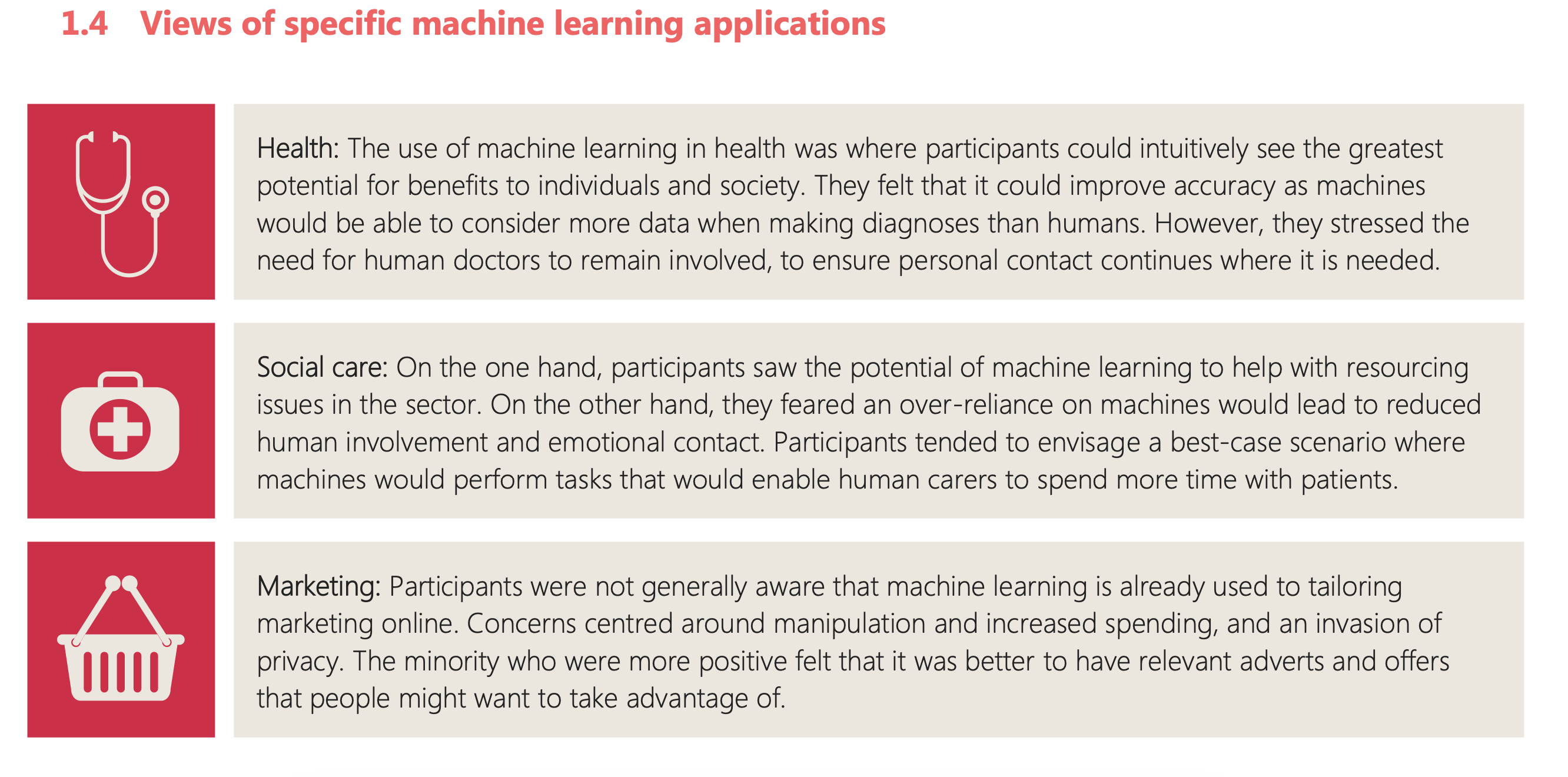
Figure: One of the questions focussed on machine learning applications.

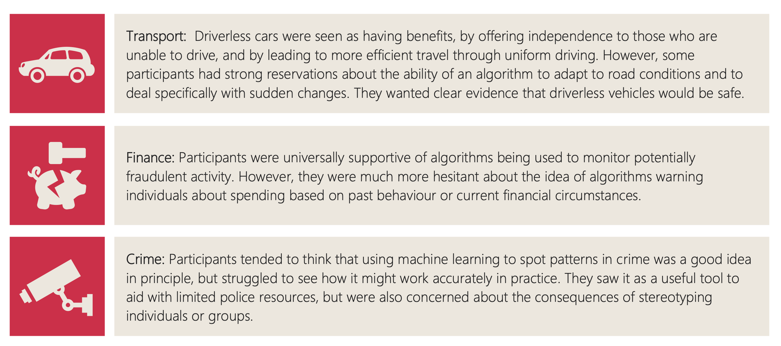
Figure: The public were broadly supportive of a range of application areas.

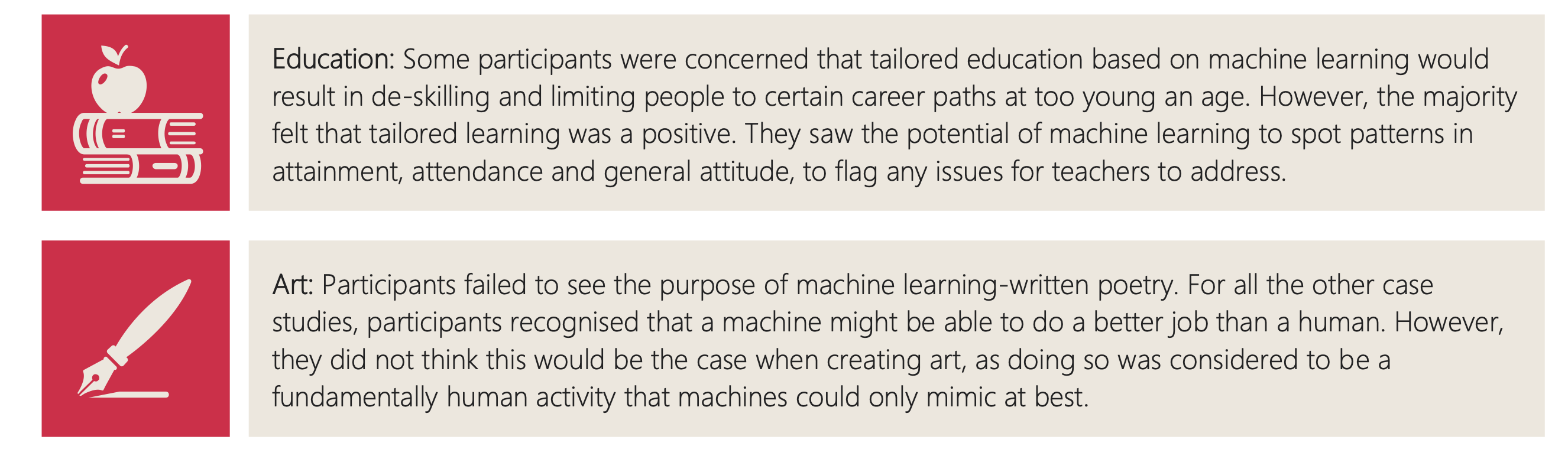
Figure: But they failed to see the point in AI’s that could produce poetry.

Probability Conversations

Figure: The focus so far has been on reducing uncertainty to a few representative values and sharing numbers with human beings. We forget that most people can be confused by basic probabilities for example the prosecutor’s fallacy.

In practice we know that probabilities can be very unintuitive, for example in court there is a fallacy known as the “prosecutor’s fallacy” that confuses conditional probabilities. This can cause problems in jury trials (Thompson, 1989).

Networked Interactions

Our modern society intertwines the machine with human interactions. The key question is who has control over these interfaces between humans and machines.

Figure: Humans and computers interacting should be a major focus of our research and engineering efforts.

So the real challenge that we face for society is understanding which systemic interventions will encourage the right interactions between the humans and the machine at all of these interfaces.

Figure: Humans use culture, facts and ‘artefacts’ to communicate.

Human Analogue Machine

The machine learning systems we have built today that can reconstruct human text, or human classification of images, necessarily must have some aspects to them that are analagous to our understanding. As MacKay suggests the brain is neither a digital or an analogue computer, and the same can be said of the modern neural network systems that are being tagged as “artificial intelligence”.

I believe a better term for them is “human-analogue machines”, because what we have built is not a system that can make intelligent decisions from first principles (a rational approach) but one that observes how humans have made decisions through our data and reconstructs that process. Machine learning is more empiricist than rational, but now we n empirical approach that distils our evolved intelligence.

Figure: The human analogue machine creates a feature space which is analagous to that we use to reason, one way of doing this is to have a machine attempt to compress all human generated text in an auto-regressive manner.

Further Reading

• Chapter 1 of Lawrence (2024)

• Chapter 11 of Lawrence (2024)

• Chapter 8 of Lawrence (2024)

The perils of developing this capability include counterfeit people, a notion that the philosopher Daniel Dennett has described in The Atlantic. This is where computers can represent themselves as human and fool people into doing things on that basis.

LLM Conversations

Figure: The focus so far has been on reducing uncertainty to a few representative values and sharing numbers with human beings. We forget that most people can be confused by basic probabilities for example the prosecutor’s fallacy.

Figure: The Inner Monologue paper suggests using LLMs for robotic planning (Huang et al., 2023).

By interacting directly with machines that have an understanding of human cultural context, it should be possible to share the nature of uncertainty in the same way humans do. See for example the paper Inner Monologue: Embodied Reasoning through Planning Huang et al. (2023).

HAM

Figure: The trinity of human, data, and computer, and highlights the modern phenomenon. The communication channel between computer and data now has an extremely high bandwidth. The channel between human and computer and the channel between data and human is narrow. New direction of information flow, information is reaching us mediated by the computer. The focus on classical statistics reflected the importance of the direct communication between human and data. The modern challenges of data science emerge when that relationship is being mediated by the machine.

Figure: The HAM now sits between us and the traditional digital computer.

AI@Cam

AI@Cam is a new flagship University mission that seeks to address these challenges. It recognises that development of safe and effective AI-enabled innovations requires this mix of expertise from across research domains, businesses, policy-makers, civill society, and from affected communities. AI@Cam is setting out a vision for AI-enabled innovation that benefits science, citizens and society.

This vision will be achieved through leveraging the University’s vibrant interdisciplinary research community. AI@Cam will form partnerships between researchers, practitioners, and affected communities that embed equity and inclusion. It will develop new platforms for innovation and knowledge transfer. It will deliver innovative interdisciplinary teaching and learning for students, researchers, and professionals. It will build strong connections between the University and national AI priorities.

The University operates as both an engine of AI-enabled innovation and steward of those innovations.

AI is not a universal remedy. It is a set of tools, techniques and practices that correctly deployed can be leveraged to deliver societal benefit and mitigate social harm.

In that sense AI@Cam’s mission is close in spirit to that of Panacea’s elder sister Hygeia. It is focussed on building and maintaining the hygiene of a robust and equitable AI research ecosystem.

Figure: AI@Cam is a Flagship Programme that supports AI research across the University.

Finally, we are working across the University to empower the diversity ofexpertise and capability we have to focus on these broad societal problems. We will recently launched AI@Cam with a vision document that outlines these challenges for the University.

The initiative was funded in November 2022 where a £5M investment from the University was secured.

Progress so far:

• Developing the vision
  • Engaged over 100 members of the University community across 30 departments/institutes, start-ups, and large businesses.
  • Supported 6 new funding bids

Conclusion

See the Gorilla don’t be the Gorilla.

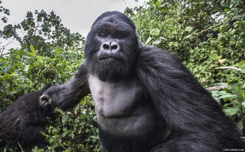
Figure: A famous quote from Mike Tyson before his fight with Evander Holyfield: “Everyone has a plan until they get punched in the mouth”. Don’t let the gorilla punch you in the mouth. See the gorilla, but don’t be the gorilla. Photo credit: https://www.catersnews.com/stories/animals/go-ape-unlucky-photographer-gets-punched-by-lairy-gorilla-drunk-from-eating-bamboo-shoots/

Thanks!

For more information on these subjects and more you might want to check the following resources.

• twitter: @lawrennd
• podcast: The Talking Machines
• newspaper: Guardian Profile Page
• blog: http://inverseprobability.com