Links

Justice: What’s The Right Thing to Do?

Figure: Sandel’s book looks at how to do the right thing with a context of moreal philosophy. Sandel (2010)

In the book “Justice: What’s The Right Thing to Do?” (Sandel, 2010) Michael Sandel aims to help us answer questions about how to do the right thing by giving some context and background in moral philosophy. Sandel is a philosopher based at Harvard University who is reknowned for his popular treatments of the subject. He starts by illustrating decision making through the ‘trolley’ problem.

The Trolley Problem

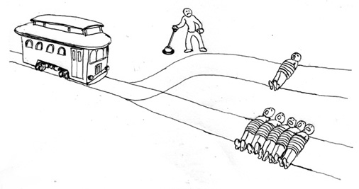
Figure: The trolley problem in its original form.

The trolley problem has become a mainstay of debates around driverless cards and is often rather crudely used, but it is more subtly wielded in is introduction by Foot (1967) where it is used as part of her analysis of the doctrine of double effect where actions have results that are not intended (oblique intention).

In the world of science, utilitarianism as a philosophy maps onto what we think of as utility theory. The assumption is that the quality of any decision can be evaluated mathematically.

This gives us an approach to balancing between the sensitivity and the specificity of any decision. The basic approach is to define a utility function, which defines the worth of different outcomes.

In machine learning this utility function maps onto what we think of as the objective function (also known as the loss, the cost function or the error function).

The Push and the Trolley

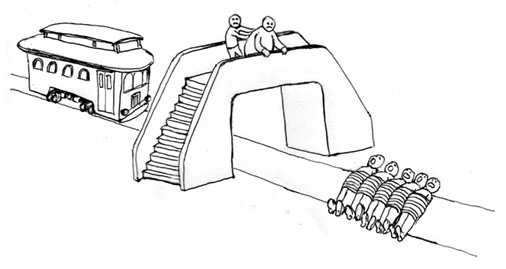
Figure: In the situation where you push an overweight gentleman, the decision is riddled with uncertainty. Doubt inevitably creeps in.

In Thomson (1976) a variation on Foot’s original formulation is considered which is allowing us to see the challenge from a transplant surgeon’s perspective: Thomson knowingly contrives a variation of the problem which is similar to the idea that a transplant surgeon should harvest organs to save the lives of five people.

Prospect Theory

Daniel Kahneman won the Nobel Memorial Prize for work on the idea of prospect theory. The theory is based on empirical studies around how humans make decisions, and suggests that not only are they sensitive to change of circumstance, rather than absolute circumstance, there is an asymmetry to the sensitivity associated with negative and positive changes.

Kahneman (2011) was a book that presented this idea but also popularised the notion of dual process cognition: where thoughts are separated into fast thinking and slow thinking. In the history of the philosophy of ethics, an ethical decision has always been associated with intentional or reflective actions. Sylvie Delacroix’s book Habitual Ethics (Delacroix, 2022) establishes the case for a theory of ethics arising from habitual (presumably fast-thinking) decisions.

Subjective Utility

Jeremy Bentham’s ideas around maximising happiness are focussed on the ide of a global utility, but natural selection suggests that there should be variation in the population, otherwise there will be no separation between effective and ineffective strategies. So in practice utilities (if they exist) must be subjective, they would vary from individual to individual.

A Cognitive Bias towards Variance

Kahneman’s book explores various ways in which humans might be considered “irrational”, for example our tendency to produce overcomplicated explanations. If prediction is of the form \[ \text{model} + \text{data} \rightarrow \text{prediction}\] then Kahneman explores the seemingly reasonable proposal that predictions from different experts should be consistent. After all, how could the predictions be correct if they are inconsistent. From a statistical perspective, simpler models tend to be more consistent. So this suggests to Kahneman that humans overcomplicate. However, once we accept that errors will be made (e.g. due to uncertainty) then we can notice that a push for consistency is a push for consistency of error.

Bias vs Variance

One way of looking at this technically in machine learning is to decompose our generalization error into two parts. The bias-variance dilemma emerges from looking at these two parts and observing that part of our error comes from oversimplification in our model (the bias error) and part of our error comes from the fact that there’s insufficient data to pin down the parameters of a more complex model (the variance error).

In Machine Learning

In the past (before the neural network revolution!) there were two principle approaches to resolving the bias-variance dilemma. Either you use over simple models, which lead to better consistency in their generalization and well determined parameters. Or you use more complex models and make use of some form of averaging to deal with the variance.

• Two approaches
  • Use simpler models (better consistency and good generalization)
  • Use more complex models and average to remove variance.

Bias vs Variance Error Plots

Helper function for sampling data from two different classes.

import numpy as np

Helper function for plotting the decision boundary of the SVM.

import urllib.request

urllib.request.urlretrieve('https://raw.githubusercontent.com/lawrennd/talks/gh-pages/mlai.py','mlai.py')

import matplotlib
font = {'family' : 'sans',
        'weight' : 'bold',
        'size'   : 22}

matplotlib.rc('font', **font)
import matplotlib.pyplot as plt

from sklearn import svm

# Create an instance of SVM and fit the data. 
C = 100.0  # SVM regularization parameter
gammas = [0.001, 0.01, 0.1, 1]


per_class=30
num_samps = 20
# Set-up 2x2 grid for plotting.
fig, ax = plt.subplots(1, 4, figsize=(10,3))
xlim=None
ylim=None
for samp in range(num_samps):
    X, y=create_data(per_class)
    models = []
    titles = []
    for gamma in gammas:
        models.append(svm.SVC(kernel='rbf', gamma=gamma, C=C))
        titles.append('$\gamma={}$'.format(gamma))
    models = (cl.fit(X, y) for cl in models)
    xlim, ylim = decision_boundary_plot(models, X, y, 
                           axs=ax, 
                           filename='bias-variance{samp:0>3}.svg'.format(samp=samp), 
                           directory='./ml'
                           titles=titles,
                          xlim=xlim,
                          ylim=ylim)

%pip install pods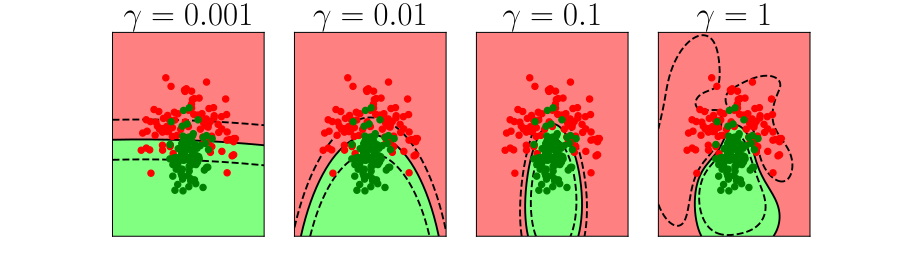

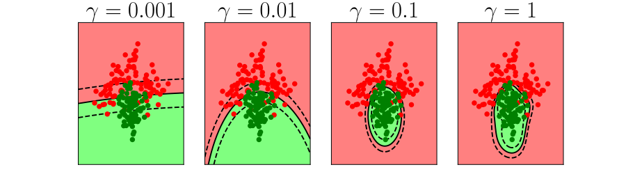
Figure: In each figure the simpler model is on the left, and the more complex model is on the right. Each fit is done to a different version of the data set. The simpler model is more consistent in its errors (bias error), whereas the more complex model is varying in its errors (variance error).

Decision Making and Bias-Variance

However in a population, where there are many decision makers, I would argue we should always err towards variance error rather than bias. This is because the averaging effects occur naturally, and we don’t have large sections of the population making consistent errors.

In practice averaging of variance errors is also prosed by Breiman and is called bagging (Breiman, 1996). (Another ensemble method that works with biased models is called boosting.

Rational Behaviour

My argument is that rational behviour requires variation. That it allows us to sustain a variety of approaches to life. That there is no single utility that we should all be optimising.

{So the observations that humans “over complicate” whether it’s in football punditry or as Meehl (1954) observes in clinical prediction, is associated with

One Correct Solution

The idea that there is one solution and that we can somehow have access to it has led to some of the horrors of science. For example, in eugenics, the notion of artificial selection (where some aspect(s) of a species is/are selected and accentuated through artifical breeding) is applied to humans. Disregarding the natural moral repulsion this engenders, it also betrays some simplistic misunderstandings of the process of evolution. What is OK for greyhounds, wheat breeds, race horses, sheep and cows is not OK for humans.

I may not agree with many people’s subjective approach to life, I may even believe it to be severely sub-optimal. But I should not presume to know better, even if prior experience shows that my own ‘way of being’ is effective.

Variation is vitally important for robustness. There may be future circumstances where my approaches fail utterly, and other ways of being are better.

If we do all have different approaches to life, then in the long run the quality of these approaches is measured by a effectiveness (which will also owe a lot to luck). From a species persistence perspective, each of these approaches is one component in our make up. The notion of a universl utility by which we are all judged is difficult (or impossible) to define.

The Real Ethical Dilemma

For driverless cars, the trolley problem is an oversimplificiation, because when people are killed it will not be through “reflective decisions” that those deaths occur, but through a consipiracy of happenstance events.

That does not mean there are no ethical dilemmas, any automation technology will have uneven effects across society. So, for example, it may be that introducing driverless cars we achieve a 90% reduction in deaths. But what if all those that now die are cyclists?

Artificial vs Natural Systems

Let’s take a step back from artificial intelligence, and consider natural intelligence. Or even more generally, let’s consider the contrast between an artificial system and an natural system. The key difference between the two is that artificial systems are designed whereas natural systems are evolved.

Systems design is a major component of all Engineering disciplines. The details differ, but there is a single common theme: achieve your objective with the minimal use of resources to do the job. That provides efficiency. The engineering designer imagines a solution that requires the minimal set of components to achieve the result. A water pump has one route through the pump. That minimises the number of components needed. Redundancy is introduced only in safety critical systems, such as aircraft control systems. Students of biology, however, will be aware that in nature system-redundancy is everywhere. Redundancy leads to robustness. For an organism to survive in an evolving environment it must first be robust, then it can consider how to be efficient. Indeed, organisms that evolve to be too efficient at a particular task, like those that occupy a niche environment, are particularly vulnerable to extinction.

This notion is akin to the idea that only the best will survive, popularly encoded into an notion of evolution by Herbert Spencer’s quote.

Survival of the fittest

Herbet Spencer, 1864

Darwin himself never said “Survival of the Fittest” he talked about evolution by natural selection.

Non-survival of the non-fit

Evolution is better described as “non-survival of the non-fit”. You don’t have to be the fittest to survive, you just need to avoid the pitfalls of life. This is the first priority.

So it is with natural vs artificial intelligences. Any natural intelligence that was not robust to changes in its external environment would not survive, and therefore not reproduce. In contrast the artificial intelligences we produce are designed to be efficient at one specific task: control, computation, playing chess. They are fragile.

The first rule of a natural system is not be intelligent, it is “don’t be stupid”.

A mistake we make in the design of our systems is to equate fitness with the objective function, and to assume it is known and static. In practice, a real environment would have an evolving fitness function which would be unknown at any given time.

You can also read this blog post on Natural and Artificial Intelligence..

The first criterion of a natural intelligence is don’t fail, not because it has a will or intent of its own, but because if it had failed it wouldn’t have stood the test of time. It would no longer exist. In contrast, the mantra for artificial systems is to be more efficient. Our artificial systems are often given a single objective (in machine learning it is encoded in a mathematical function) and they aim to achieve that objective efficiently. These are different characteristics. Even if we wanted to incorporate don’t fail in some form, it is difficult to design for. To design for “don’t fail”, you have to consider every which way in which things can go wrong, if you miss one you fail. These cases are sometimes called corner cases. But in a real, uncontrolled environment, almost everything is a corner. It is difficult to imagine everything that can happen. This is why most of our automated systems operate in controlled environments, for example in a factory, or on a set of rails. Deploying automated systems in an uncontrolled environment requires a different approach to systems design. One that accounts for uncertainty in the environment and is robust to unforeseen circumstances.

Uncertainty and Absolutism

One of the most understood aspects of evolution is the idea that evolution is survival of the fittest. It’s better described of non-survival of the non-fit, and what fit even means is highly subjective. Any utility function evolves socially andwith our environment. “Survival of the fittest” is not due to Darwin it’s associated with Herbert Spencer and closely associated with social Darwinism which has little to do with the way that evolution operates in practice.

Absolute Policies

Because of these uncertainties there’s an emergent rule:

There will be no single absolute policy that should be followed slavishly in all circumstances

This is also acknowledged in the field of statistics, most famously in the quote by George Box.

Some Models are Useful

So, when do we fall outside this important domain where we have the correct model? According to Box (1976), all the time.

All models are wrong, but some are useful

Box’s important quote has become worn by overuse (like a favorite sweater). Indeed, I most often see it quoted at the beginning of a talk in a way that confuses correlation with causality. Presentations proceed in the following way. (1) Here is my model. (2) It is wrong. (3) Here is George Box’s quote. (4) My model is wrong, but it might be useful. Sometimes I feel at stage (4) a confusion about the arrow of causality occurs, it feels to me that people are almost saying “Because my model is wrong it might be useful.”

Perhaps we should be more focusing on the quote from the same paper¹

Since all models are wrong the scientist must be alert to what is importantly wrong. It is inappropriate to be concerned about mice when there are tigers abroad.

George E. P. Box (Box, 1976)

Tigers and Trolleys

In the world of trolley problems this perhaps maps best to the version of the problem where to save the lives of five people you have to push a large gentleman off a bridge.

Uncertainty: The Tyger that Burns Bright

Tyter Tyger, burning bright, In the forests of the night; What immortal hand or eye, Could frame thy fearful symmetry?

First verse of The Tyger by William Blake, 1794

A major challenge with this notion of utility is the assumption that we can describe our objectives mathematically. Once this notion is challenged some severe weaknesses in the way we do machine learning can be seen to emerge.

Thanks!

For more information on these subjects and more you might want to check the following resources.

• book: The Atomic Human
• twitter: @lawrennd
• podcast: The Talking Machines
• newspaper: Guardian Profile Page
• blog: http://inverseprobability.com

References