My Background

I’d like to start this talk by emphasizing that I don’t know anything about emergency medicine, except what I picked up by cycling with a friend who works in A&E in Rotherham.

So as far as I’m aware, all emergency medicine doctors are extremely good cyclists.

What I do know about is deployments of machine learning, how they succeed, how they fail. Both from a manager’s perspective, a domain expert’s perspective and a user’s perspective. For our context, let’s map these people onto the senior administrator, the doctors and nurses and the patients.

Artificial Intelligence

Let’s start with the term artificial intelligence. It’s an extremely emotive term because intelligence is something precious to us. It implies that the machine is encroaching on territory which we formerly thought of as our own.

Anthrox

The emotive nature of the term is not the only problem, the second problem with the term is anthrox. In the word anthrox the X stands for pomorphisation. So the full word is normally anthropomorphisation.

We are bandwidth limited, so when interacting with other intelligent agents, we make assumptions that they think and operate like us. That is the tendency to anthrox. The problem is pernicious because it’s difficult to say, so we tend not to call it out in case our tongue trips us up. That’s why we’ll call it anthtrox. When communicating with humans, anthrox is a short cut to gaining a form of information coherence of what your objectives are. You can use contextual analogies to align activities. You don’t need to send detailed and explicit instructions. You can rely on your team of professionals to work towards one goal, making the patient safe and comfortable. All of this is implicit in the humans around you. It cannot be taken forgranted in the computer.

Bandwidth Constrained Conversations

Figure: Conversation relies on internal models of other individuals.

Figure: Misunderstanding of context and who we are talking to leads to arguments.

Embodiment factors imply that, in our communication between humans, what is not said is, perhaps, more important than what is said. To communicate with each other we need to have a model of who each of us are.

To aid this, in society, we are required to perform roles. Whether as a parent, a teacher, an employee or a boss. Each of these roles requires that we conform to certain standards of behaviour to facilitate communication between ourselves.

Control of self is vitally important to these communications.

The high availability of data available to humans undermines human-to-human communication channels by providing new routes to undermining our control of self.

If you must anthrox AI, then please think of it as an extremely literal and willful friend, who ignores social cues. Is the last to remain at the party, will blurt out the most inappropriate conclusions regardless of the social context. Has an encyclopedic knowledge about things that sound irrelevant to you.

The truth is that the current generation of artificial intelligence solutions are almost entirely based on machine learning, and machine learning is simply a combination of compute and statistics. So it will help you a great deal if whenever you see the term AI, you mentally replace it with computers and statistics. That will give you a more realistic understanding of its capabilities.

Bandwidth Constrained Conversations

Figure: Conversation relies on internal models of other individuals.

Figure: Misunderstanding of context and who we are talking to leads to arguments.

Embodiment factors imply that, in our communication between humans, what is not said is, perhaps, more important than what is said. To communicate with each other we need to have a model of who each of us are.

To aid this, in society, we are required to perform roles. Whether as a parent, a teacher, an employee or a boss. Each of these roles requires that we conform to certain standards of behaviour to facilitate communication between ourselves.

Control of self is vitally important to these communications.

The high availability of data available to humans undermines human-to-human communication channels by providing new routes to undermining our control of self.

A particular bias that is important is automation bias

I was skimming a recent nature paper about these techniques in medicine, a paper that used machine learning to classify potentially cancerous images. Throuhout the paper they refer to an ‘AI system.’ Whether it is conscious or not, the paper plays on our tendency to anthrox. It makes the work feel like it’s doing something magical, that it relates to our intelligence. This is a particularly dangerous trap for a medical professional to fall into.

Managers see AI as a way of improving processes and giving them more control over decision making in their organisation. People are hard to control, computers are easy to control.

Domain experts have an understanding of context of decisions, and an intuition about what the right decision might be. But they can be blind to unusual situations and overly convinced by their own expertise.

Users are placing trust in the decision making process. They want to believe in the outcome, and like to think that it considers there personal circumstances and that it is fair in some way.

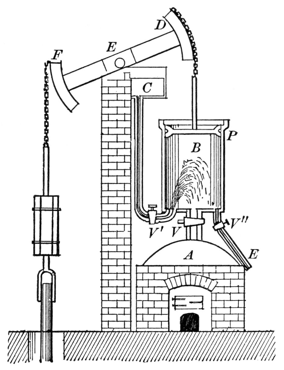
Figure: Thomas Newcomen’s steam engine predated James’ Watt’s by 60 years, but it was inefficient because it relied on a cooling of the cylinder by direct injection of water. Watt realised this was inefficient and developed the separate condensor.

The promise of artificial intelligence is that it is the first generation of automation that will adapt to us rather than us adapting to it. What do I mean by that? The challenges of automation are not new. In the 18th century, automation of the physical labour of pumping mines clear of water was a priority, and the steam engine was invented and evolved for that task. The challenge is that the engine is not flexible, it is designed to do one job repetitively. It is like a small baby. It needs feeding, it needs cleaning, and it has regular emissions. It has no concept of time or convenience of those that maintain it.

Although the computer is more advanced than the steam engine in many respects, it is still utterly dependent on its human operators. For the information it gets in the form of data (the input coal) to the actions it takes in response (the operation of the mine pump). It doesn’t have a contextual awareness of side effects of those decisions because they don’t fall within its cognitive landscape. Just like the steam engine, it doesn’t wear nappies, so any unaccounted for side effects of feeding it with data are felt by the environment.

Figure: Machines are as helpless and unaware as small children, and less cute. Just like a small child they require us to maintain and service them.

Figure: Steen’s painting of the doctor and patient reminds us that bedside manner is a critical component of the relationship.

Figure: When we deploy at scale the damage done by deploying a naive machine can feel exactly like the damage done by deploying a maliscious machine.

The machine is also relentless, as long as it is fed, it can complete actions tirelessly, day or night.

Having said that, it’s remarkable what we’re doing today with computers and statistics. And the drive for this is really the quantity of data available. In particular we have significant advances in what we might think of as tasks that traditionally needed human perception to solve. For example, object detection in images. We can now train computers to identify and highlight objects that a decade ago were only identifiable by humans.

How have we achieved this?

Deep Learning

DeepFace

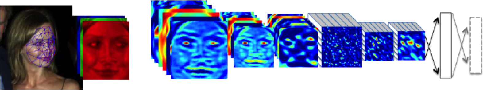
Figure: The DeepFace architecture (Taigman et al., 2014), visualized through colors to represent the functional mappings at each layer. There are 120 million parameters in the model.

The DeepFace architecture (Taigman et al., 2014) consists of layers that deal with translation invariances, known as convolutional layers. These layers are followed by three locally-connected layers and two fully-connected layers. Color illustrates feature maps produced at each layer. The neural network includes more than 120 million parameters, where more than 95% come from the local and fully connected layers.

Deep Learning as Pinball

Figure: Deep learning models are composition of simple functions. We can think of a pinball machine as an analogy. Each layer of pins corresponds to one of the layers of functions in the model. Input data is represented by the location of the ball from left to right when it is dropped in from the top. Output class comes from the position of the ball as it leaves the pins at the bottom.

Sometimes deep learning models are described as being like the brain, or too complex to understand, but one analogy I find useful to help the gist of these models is to think of them as being similar to early pin ball machines.

In a deep neural network, we input a number (or numbers), whereas in pinball, we input a ball.

Think of the location of the ball on the left-right axis as a single number. Our simple pinball machine can only take one number at a time. As the ball falls through the machine, each layer of pins can be thought of as a different layer of ‘neurons.’ Each layer acts to move the ball from left to right.

In a pinball machine, when the ball gets to the bottom it might fall into a hole defining a score, in a neural network, that is equivalent to the decision: a classification of the input object.

An image has more than one number associated with it, so it is like playing pinball in a hyper-space.

Figure: At initialization, the pins, which represent the parameters of the function, aren’t in the right place to bring the balls to the correct decisions.

Figure: After learning the pins are now in the right place to bring the balls to the correct decisions.

Learning involves moving all the pins to be in the correct position, so that the ball ends up in the right place when it’s fallen through the machine. But moving all these pins in hyperspace can be difficult.

In a hyper-space you have to put a lot of data through the machine for to explore the positions of all the pins. Even when you feed many millions of data points through the machine, there are likely to be regions in the hyper-space where no ball has passed. When future test data passes through the machine in a new route unusual things can happen.

Adversarial examples exploit this high dimensional space. If you have access to the pinball machine, you can use gradient methods to find a position for the ball in the hyper space where the image looks like one thing, but will be classified as another.

Probabilistic methods explore more of the space by considering a range of possible paths for the ball through the machine. This helps to make them more data efficient and gives some robustness to adversarial examples.

Similar comments could be made for machine learning systems that are recognising speech (e.g. in voice assistances such as Siri, Alexa and Google Assistant). And for automated language translation. However, these systems are critically dependent on our data, on data that has been labelled by humans. They are emulating our perceptual set up through having observed lare amounts of data.

On average we may be able to show that these machines outperform us, but this also can bring problems. It turns out to be important not just whether we are wrong, but how we are wrong.

Boulton and Watt’s Steam Engine

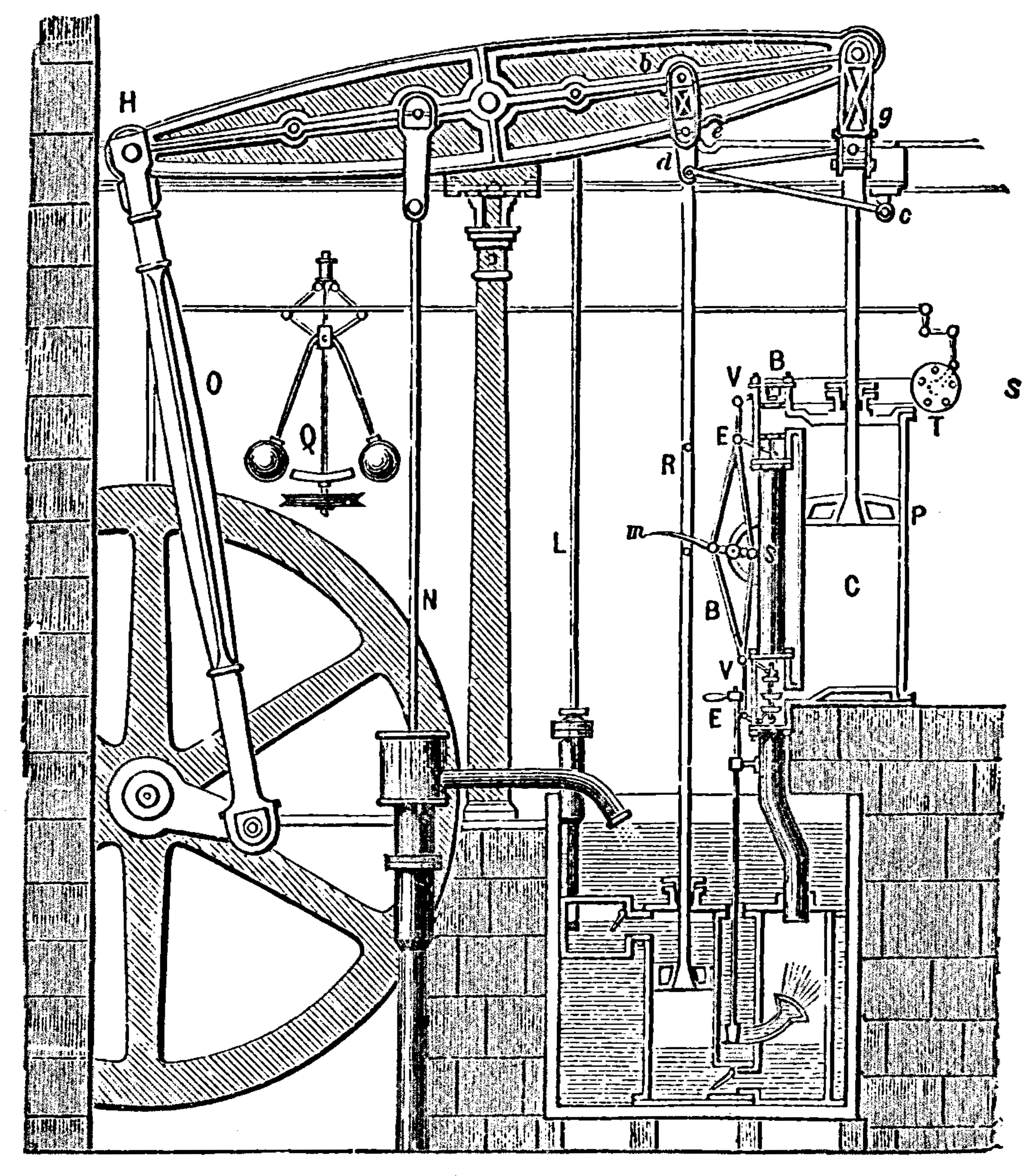
Figure: Watt’s Steam Engine which made Steam Power Efficient and Practical.

James Watt’s steam engine contained an early machine learning device. In the same way that modern systems are component based, his engine was composed of components. One of which is a speed regulator sometimes known as Watt’s governor. The two balls in the center of the image, when spun fast, rise, and through a linkage mechanism.

Bias vs Variance Error Plots

Helper function for sampling data from two different classes.

import numpy as np

Helper function for plotting the decision boundary of the SVM.

import urllib.request

urllib.request.urlretrieve('https://raw.githubusercontent.com/lawrennd/talks/gh-pages/mlai.py','mlai.py')

import matplotlib
font = {'family' : 'sans',
        'weight' : 'bold',
        'size'   : 22}

matplotlib.rc('font', **font)
import matplotlib.pyplot as plt

from sklearn import svm

# Create an instance of SVM and fit the data. 
C = 100.0  # SVM regularization parameter
gammas = [0.001, 0.01, 0.1, 1]


per_class=30
num_samps = 20
# Set-up 2x2 grid for plotting.
fig, ax = plt.subplots(1, 4, figsize=(10,3))
xlim=None
ylim=None
for samp in range(num_samps):
    X, y=create_data(per_class)
    models = []
    titles = []
    for gamma in gammas:
        models.append(svm.SVC(kernel='rbf', gamma=gamma, C=C))
        titles.append('$\gamma={}$'.format(gamma))
    models = (cl.fit(X, y) for cl in models)
    xlim, ylim = decision_boundary_plot(models, X, y, 
                           axs=ax, 
                           filename='bias-variance{samp:0>3}.svg'.format(samp=samp), 
                           directory='./ml'
                           titles=titles,
                          xlim=xlim,
                          ylim=ylim)

%pip install pods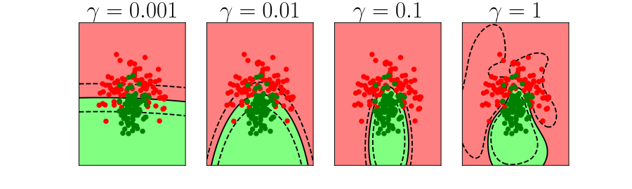

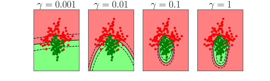
Figure: In each figure the simpler model is on the left, and the more complex model is on the right. Each fit is done to a different version of the data set. The simpler model is more consistent in its errors (bias error), whereas the more complex model is varying in its errors (variance error).

One of the very real problems we face at the moment is we have an ecosystem of people and companies that are delivering solutions that are not driven by the ‘pain points’ of our health service, not driven by getting the fundamentals right. Not driven by solutions that would make a difference for patients, doctors, nurses and administrators but driven by headlines. These are companies that are not making money from these solutions, but are engaged in a wider battle for mindshare. To give the impression that AI systems are delivering magical solutions.

It’s an intrinsic part of their agenda because in the near term this is the fastest route to large scale investment. Capturing the imagination of the public, investors, vice-presidents and CEOs is a far surer route to a billion dollar check than actually trying to build and deploy a product in such a complex ecosystem as the healthcare market.

But we shouldn’t bemoan this too much. This stage is likely inevitable, but it is unsustainable. The key question is, how do we take advantage of the excitement to deliver sustainable change that benefits all doctors?

Many of the particular answers to this are personal, but here’s a couple of ideas I think might help. Firstly, it’s a learning opportunity. First, you should assimilate the skepticism, but once you’ve understood the very real reasons why there won’t be overnight success, then you should indulge your curiousity, and allow the child in you to emerge. There are fascinating technologies emerging, and the current excitement means there will be more opportunities to learn about these technologies and inspire you to think about how they might make your life easier. But then you need to take off the rose-tinted spectacles and examine how such technologies might be making a difference in your particular A&E. How does this neural network change the life of the metal worker from Rotherham with a steel splint in her eye? Because if that question isn’t being asked, then the applicability of the technology is not being considered. The benefit may of course be indirect, but if it is not eventually felt by patients in some way then the utility is questionable.

Secondly, to deploy any of these systems you will find that the main barriers are in your existing processes. A classic mistake is to believe that you can bring in an advanced machine learning technique and deploy it within your hospital environment, when the reality is that the machine will face all the challenges you face and more. In particular, given that the machine is making decisions on the basis of data that you provide, how does it get access to that data? How do you ensure that the data is of sufficient quality and consistency for the machine to make a high quality decision? How do you ensure that patient privacy is respected in the processing of that data, and that the decision isn’t biased to favour a particular group? As you face the reality of the deployment you’re considering you’ll find that the real challenges are the very poor quality of existing processes. Improving those processes will improve outcome even if you do not integrate and deploy an AI system. Making your department ‘AI ready’ is far more work than building the machine learning model.

An excellent way of considering these two challenges can be done today, without major AI expertise. If you have an idea for how AI can help you in your job, here’s my suggestion. Go back to your department and mock-it-up. Whatever decision the AI is going to take can be first taken by a human. Decide what information that human will have available. Choose something where the human is going to make a decision quickly on the basis of only the information they have in front of them. The decision should be one that can take less than a second. Now install that human in your decision making pipeline. How is that decision going to be presented to patients, nurses and doctors? What does the interface look like? Remember, you don’t get to ask the decision maker to contextualise it, you need to be able to take the decision at face value and integrate it into your existing processes.

I suspect there are very few areas where this can be usefully done in an exising A&E department. Why aren’t there more? Because currently most of the processes rely on human flexibility and ability to contextualise. They are poorly documented, and in many cases deliberately obscured in an effort to protect individual domains. The very excercise of understanding why these decisions are difficult to make can be helpful in improving processes in any organisation, and I suspect A&E departments in hospitals are no different.

It’s equivalent to turning up in a 16th century farm with an internal combustion engine. At that time in the UK¹ 58% of the labour force worked in agriculture, today 1.2% of the labour force are in agriculture. But the only people who are empowered to make this change are the domain experts. The people in this room.

Public Use of Data for Public Good

Since machine learning methods are so dependent on data, Understanding public attitudes to the use of their data is key to developing machine learning methods that maintain the trust of the public. Nowhere are the benefits of machine learning more profound, and the potential pitfalls more catastrophic than in the use of machine learning in health data.

The promise is for methods that take a personalized perspective on our individual health, but health data is some of the most sensitive data available to us. This is recognised both by the public and by regulation.

With this in mind The Wellcome Trust launched a report on “Understanding Patient Data” authored by Nicola Perrin, driven by the National Data Guardian’s recommendations.

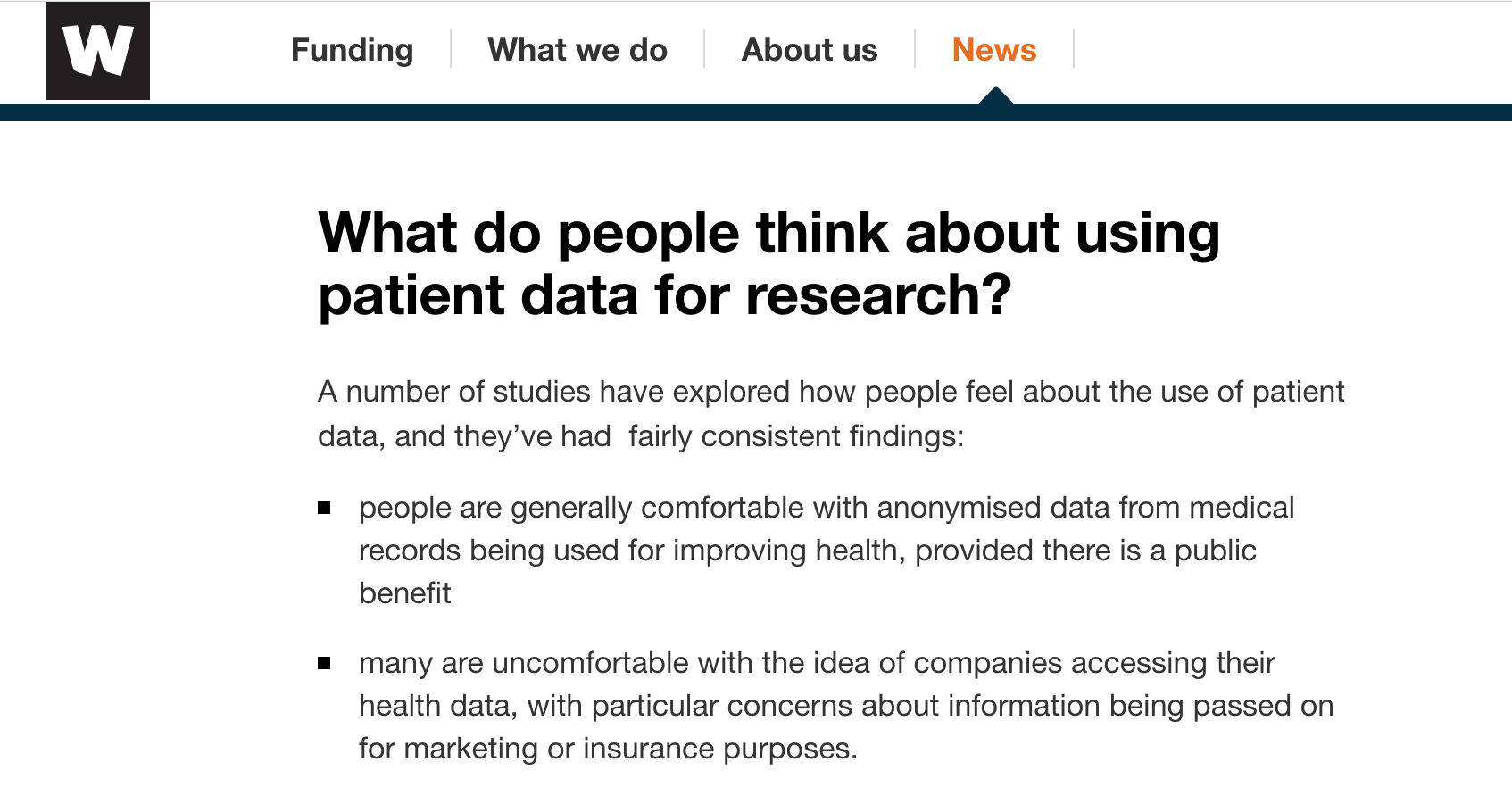
Figure: The Wellcome Trust surveyed patients to determine their attitudes to the sharing of their data.

From this report we know that patients trust Universities and hospitals more than the trust commercial entities and insurers. However, there are a number of different ways in which data can be mishandled, it is not only the intent of the data-controllers that effects our data security.

For example, the WannaCry virus attack which demonstrated the unpreparedness of much of the NHS IT infrastructure for a virus exhibiting an exploit that was well known to the security community. The key point is that the public trust the intent of academics and medical professionals, but actual capability could be at variance with the intent.

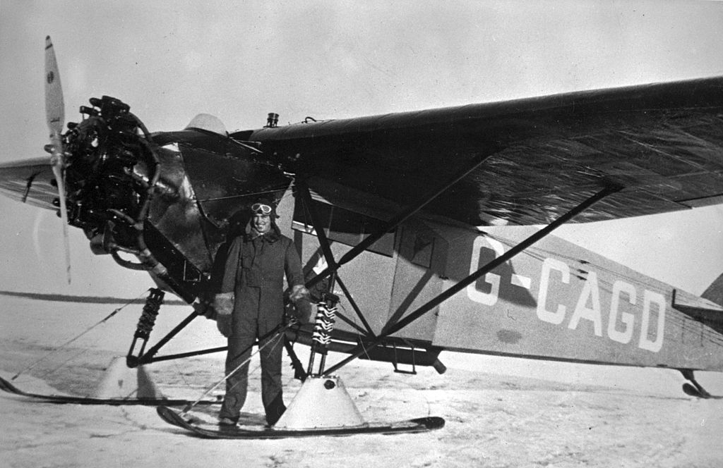
Figure: Bush Pilot Grant McConachie. A Bush Pilot is expected to fly the plane, but also to be able to repair it in difficult and isolated conditions.

The situation is somewhat reminiscient of early aviation. This is where we are with our data science capabilities. By analogy, the engine of the plane is our data security infrastructure, the basic required technology to make us safe. The pilot is the health professional performing data analytics. The nature of the job of early pilots and indeed today’s bush pilots (who fly to remote places) included a need to understand the mechanics of the engine. Just as a health data scientist, today, needs to deal with security of the infrastructure as well as the nature of the analysis.

Figure: British Airways 747 at SFO. Today airlines lease their engines from Rolls Royce who take care of maintenance independently from the pilot.

I suspect most passengers would find it disconcerting if the pilot of a 747 was seen working on the engine shortly before a flight. As aviation has become more widespread, there is now a separation of responsibilities between pilots and mechanics. For example, Rolls Royce goes so far as to maintain ownership of their engines, and lease them to the airline. The responsibility for maintenance of the engine is entirely with Rolls Royce, yet the pilot is responsibility for the safety of the aircraft and its passengers.

We need to develop a modern data-infrastructure for which separates the need for security of infrastructure from the decision making of the data analyst.

This separation of responsibility according to expertise needs to be emulated when considering health data infrastructure. This resolves the intent-capability dilemma, by ensuring a separation of responsibilities to those that are best placed to address the issues.

Figure: Black Box Thinking by Matthew Syed. Matthew compares the open approach to errors taken in the airline industry to way errors are dealt with in the health system drawing on Martin Bromiley’s experiences.

Propagation of Best Practice

We must also be careful to maintain openness in this new genaration of digital solutions across health and society. Matthew Syed’s book, Black Box Thinking (Syed, 2015), emphasizes the importance of surfacing errors as a route to learning and improved process. Taking aviation as an example, and contrasting it with the culture in medicine, Matthew relates the story of Martin Bromiley, an airline pilot whose wife died during a routine hospital procedure and his efforts to improve the culture of safety in medicine. The motivation for the book is the difference in culture between aviation and medicine in how errors are acknowledged and dealt with. We must ensure that these high standards of oversight apply to the era of data-driven automated decision making.

In particular, while there is much to be gained by involving commercial companies in the care of patients, if the process by which they are drawing inference about patient condition is hidden (for example, due to commercial confidentiality), this may prevent us from understanding errors in diagnosis or treatment. This would be a retrograde step. It may be that health device certification needs modification or reform for data-driven automated decision making, but we need a spirit of transparency around how these systems are deriving their inferences to ensure best practice.

Cognitive Diversity

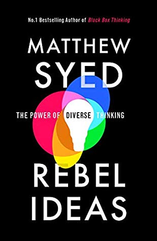
Figure: Rebel Ideas by Matthew Syed focusses on the importance of cognitive diversity in decision making. The need for diversity is a consequence of uncertainty.

Rebel Ideas focuses on the importance of diversity in problem solving (Syed, 2019). This is particularly pronounced in the presence of uncertainty. It is unlikely that there is a single person that knows all the answers, or that even a particular expertise is the only expertise you need in the room. The reality is that a range of different opinions are often required and that the better ideas often lie at the intersection of different expertise.

Thanks!

For more information on these subjects and more you might want to check the following resources.

• twitter: @lawrennd
• podcast: The Talking Machines
• newspaper: Guardian Profile Page
• blog: http://inverseprobability.com

References