Abstract

Data is not so much the new oil, it is the new software. Data driven algorithms are increasingly present in continuously deployed production software. What challenges does this present and how can the mathematical sciences help?

Introduction

Peppercorns

Figure: A peppercorn is a system design failure which is not a bug, but a conformance to design specification that causes problems when the system is deployed in the real world with mischevious and adversarial actors.

Asking Siri “What is a trillion to the power of a thousand minus one?” leads to a 30 minute response¹ consisting of only 9s. I found this out because my nine year old grabbed my phone and did it. The only way to stop Siri was to force closure. This is an interesting example of a system feature that’s not a bug, in fact it requires clever processing from Wolfram Alpha. But it’s an unexpected result from the system performing correctly.

This challenge of facing a circumstance that was unenvisaged in design but has consequences in deployment becomes far larger when the environment is uncontrolled. Or in the extreme case, where actions of the intelligent system effect the wider environment and change it.

These unforseen circumstances are likely to lead to need for much more efficient turn-around and update for our intelligent systems. Whether we are correcting for security flaws (which are bugs) or unenvisaged circumstantial challenges: an issue I’m referring to as peppercorns. Rapid deployment of system updates is required. For example, Apple have “fixed” the problem of Siri returning long numbers.

Here’s another one from Reddit, of a Tesla Model 3 system hallucinating traffic lights.

The challenge is particularly acute because of the scale at which we can deploy AI solutions. This means when something does go wrong, it may be going wrong in billions of households simultaneously.

You can also check this blog post on Decision Making and Diversity. and this blog post on Natural vs Artifical Intelligence..

Deep Learning

DeepFace

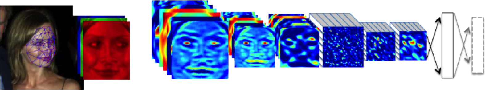
Figure: The DeepFace architecture (Taigman et al., 2014), visualized through colors to represent the functional mappings at each layer. There are 120 million parameters in the model.

The DeepFace architecture (Taigman et al., 2014) consists of layers that deal with translation and rotational invariances. These layers are followed by three locally-connected layers and two fully-connected layers. Color illustrates feature maps produced at each layer. The neural network includes more than 120 million parameters, where more than 95% come from the local and fully connected layers.

Deep Learning as Pinball

Figure: Deep learning models are composition of simple functions. We can think of a pinball machine as an analogy. Each layer of pins corresponds to one of the layers of functions in the model. Input data is represented by the location of the ball from left to right when it is dropped in from the top. Output class comes from the position of the ball as it leaves the pins at the bottom.

Sometimes deep learning models are described as being like the brain, or too complex to understand, but one analogy I find useful to help the gist of these models is to think of them as being similar to early pin ball machines.

In a deep neural network, we input a number (or numbers), whereas in pinball, we input a ball.

Think of the location of the ball on the left-right axis as a single number. Our simple pinball machine can only take one number at a time. As the ball falls through the machine, each layer of pins can be thought of as a different layer of ‘neurons.’ Each layer acts to move the ball from left to right.

In a pinball machine, when the ball gets to the bottom it might fall into a hole defining a score, in a neural network, that is equivalent to the decision: a classification of the input object.

An image has more than one number associated with it, so it is like playing pinball in a hyper-space.

%pip install pods

Figure: At initialization, the pins, which represent the parameters of the function, aren’t in the right place to bring the balls to the correct decisions.

Figure: After learning the pins are now in the right place to bring the balls to the correct decisions.

Learning involves moving all the pins to be in the correct position, so that the ball ends up in the right place when it’s fallen through the machine. But moving all these pins in hyperspace can be difficult.

In a hyper-space you have to put a lot of data through the machine for to explore the positions of all the pins. Even when you feed many millions of data points through the machine, there are likely to be regions in the hyper-space where no ball has passed. When future test data passes through the machine in a new route unusual things can happen.

Adversarial examples exploit this high dimensional space. If you have access to the pinball machine, you can use gradient methods to find a position for the ball in the hyper space where the image looks like one thing, but will be classified as another.

Probabilistic methods explore more of the space by considering a range of possible paths for the ball through the machine. This helps to make them more data efficient and gives some robustness to adversarial examples.

Containerization

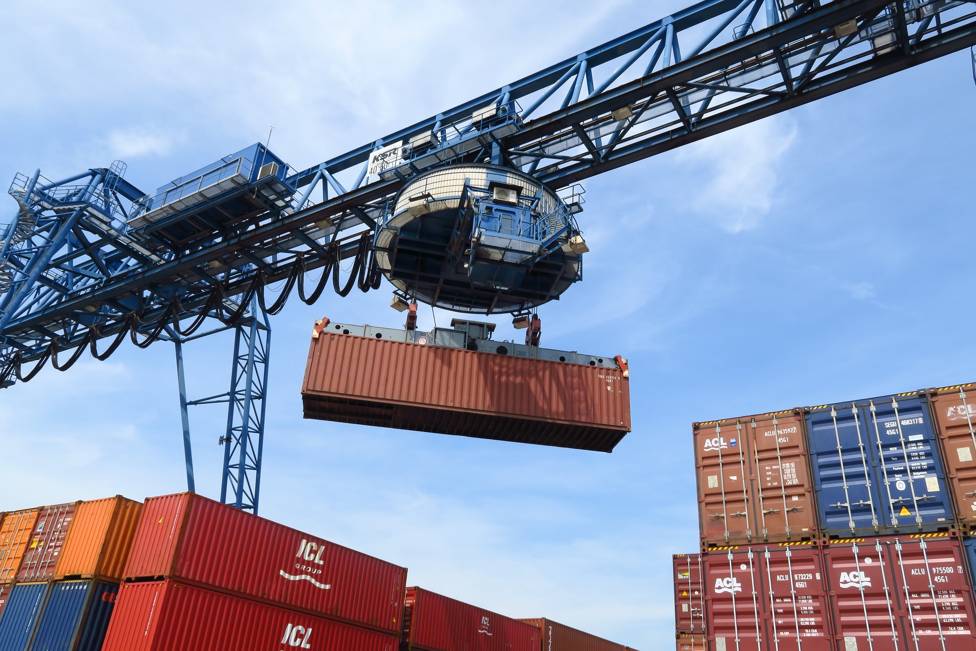
Figure: The container is one of the major drivers of globalization, and arguably the largest agent of social change in the last 100 years. It reduces the cost of transportation, significantly changing the appropriate topology of distribution networks. The container makes it possible to ship goods halfway around the world for cheaper than it costs to process those goods, leading to an extended distribution topology.

Containerization has had a dramatic effect on global economics, placing many people in the developing world at the end of the supply chain.

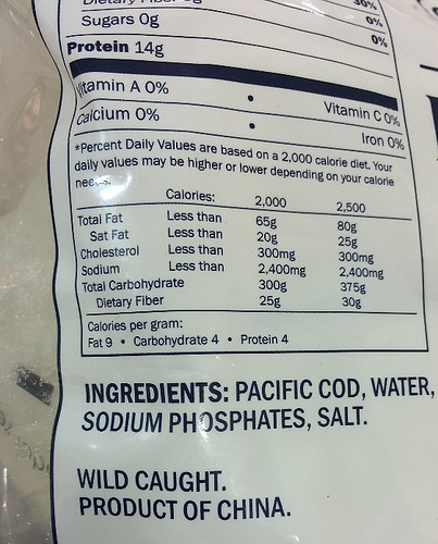
Figure: Wild Alaskan Cod, being solid in the Pacific Northwest, that is a product of China. It is cheaper to ship the deep frozen fish thousands of kilometers for processing than to process locally.

For example, you can buy Wild Alaskan Cod fished from Alaska, processed in China, sold in North America. This is driven by the low cost of transport for frozen cod vs the higher relative cost of cod processing in the US versus China. Similarly, Scottish prawns are also processed in China for sale in the UK.

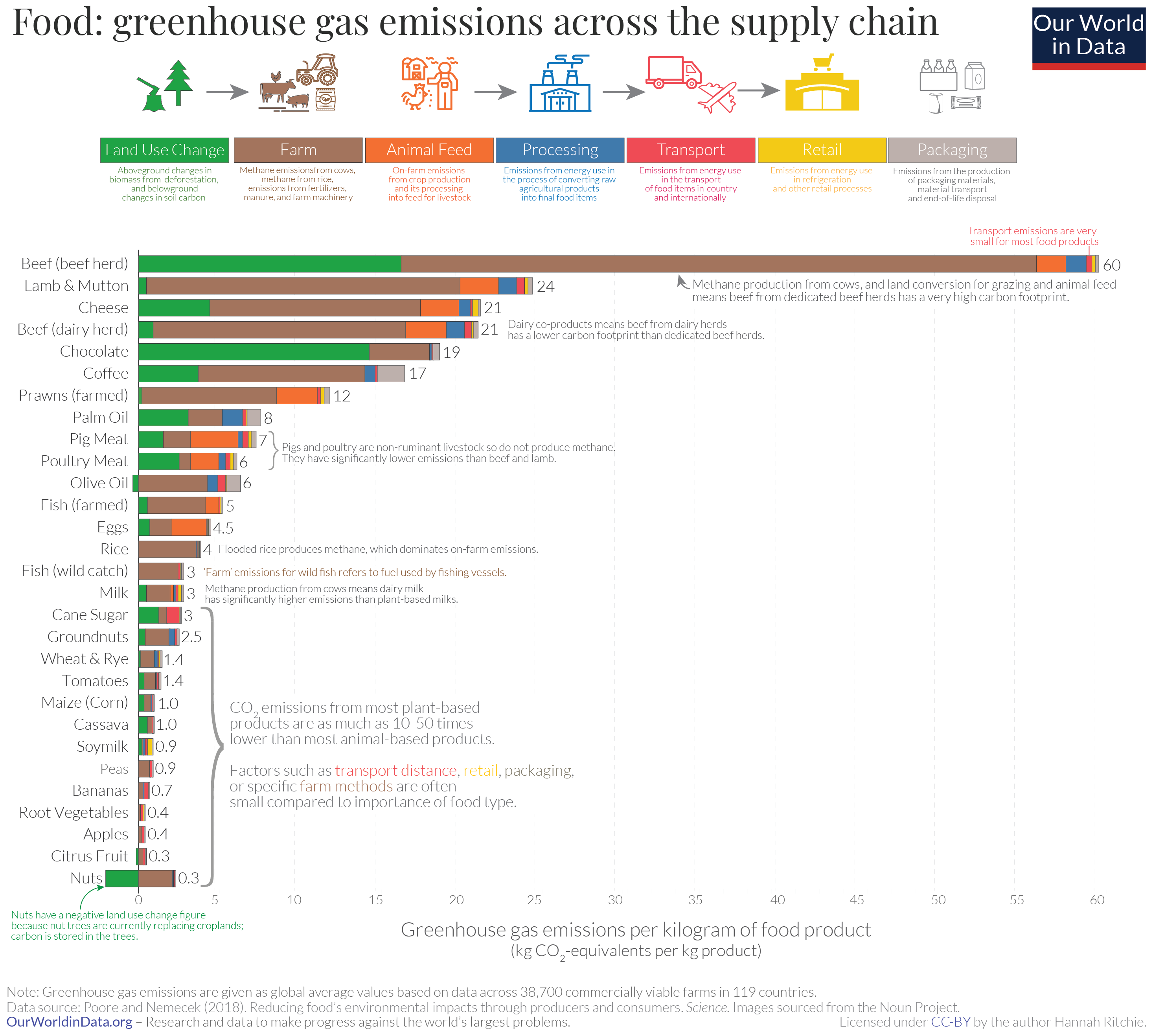
Figure: The transport cost of most foods is a very small portion of the total cost. The exception is if foods are air freighted. Source: https://ourworldindata.org/food-choice-vs-eating-local by Hannah Ritche CC-BY

This effect on cost of transport vs cost of processing is the main driver of the topology of the modern supply chain and the associated effect of globalization. If transport is much cheaper than processing, then processing will tend to agglomerate in places where processing costs can be minimized.

Large scale global economic change has principally been driven by changes in the technology that drives supply chain.

So many examples in terms of the need for intelligent decision making are based around the challenge of moving goods/energy/compute/water/medicines/drivers/people from where it is to where it needs to be. In other words matching supply with demand. That led me to a motto I developed while working in Amazon’s supply chain.

Solve Supply Chain, then solve everything else.

Statistical Emulation

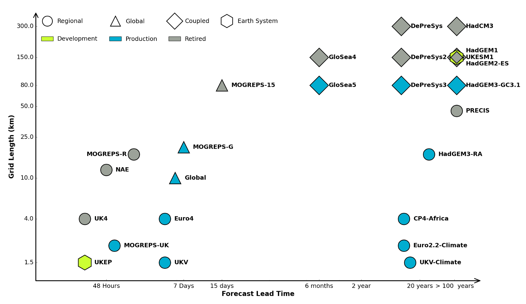
Figure: The UK Met office runs a shared code base for its simulations of climate and the weather. This plot shows the different spatial and temporal scales used.

In many real-world systems, decisions are made through simulating the environment. Simulations may operate at different granularities. For example, simulations are used in weather forecasts and climate forecasts. Interestingly, the UK Met office uses the same code for both, it has a “Unified Model” approach, but they operate climate simulations at greater spatial and temporal resolutions.

Figure: Real world systems consist of simulators that capture our domain knowledge about how our systems operate. Different simulators run at different speeds and granularities.

Figure: A statistical emulator is a system that reconstructs the simulation with a statistical model.

A statistical emulator is a data-driven model that learns about the underlying simulation. Importantly, learns with uncertainty, so it ‘knows what it doesn’t know.’ In practice, we can call the emulator in place of the simulator. If the emulator ‘doesn’t know,’ it can call the simulator for the answer.

Figure: A statistical emulator is a system that reconstructs the simulation with a statistical model. As well as reconstructing the simulation, a statistical emulator can be used to correlate with the real world.

As well as reconstructing an individual simulator, the emulator can calibrate the simulation to the real world, by monitoring differences between the simulator and real data. This allows the emulator to characterize where the simulation can be relied on, i.e., we can validate the simulator.

Similarly, the emulator can adjudicate between simulations. This is known as multi-fidelity emulation. The emulator characterizes which emulations perform well where.

If all this modelling is done with judicious handling of the uncertainty, the computational doubt, then the emulator can assist in desciding what experiment should be run next to aid a decision: should we run a simulator, in which case which one, or should we attempt to acquire data from a real-world intervention.

Uncertainty Quantification

Uncertainty quantification (UQ) is the science of quantitative characterization and reduction of uncertainties in both computational and real world applications. It tries to determine how likely certain outcomes are if some aspects of the system are not exactly known.

We will to illustrate different concepts of Uncertainty Quantification (UQ) and the role that Gaussian processes play in this field. Based on a simple simulator of a car moving between a valley and a mountain, we are going to illustrate the following concepts:

• Systems emulation. Many real world decisions are based on simulations that can be computationally very demanding. We will show how simulators can be replaced by emulators: Gaussian process models fitted on a few simulations that can be used to replace the simulator. Emulators are cheap to compute, fast to run, and always provide ways to quantify the uncertainty of how precise they are compared the original simulator.

• Emulators in optimization problems. We will show how emulators can be used to optimize black-box functions that are expensive to evaluate. This field is also called Bayesian Optimization and has gained an increasing relevance in machine learning as emulators can be used to optimize computer simulations (and machine learning algorithms) quite efficiently.

• Multi-fidelity emulation methods. In many scenarios we have simulators of different quality about the same measure of interest. In these cases the goal is to merge all sources of information under the same model so the final emulator is cheaper and more accurate than an emulator fitted only using data from the most accurate and expensive simulator.

Mountain Car Simulator

To illustrate the above mentioned concepts we use the mountain car simulator. This simulator is widely used in machine learning to test reinforcement learning algorithms. The goal is to define a control policy on a car whose objective is to climb a mountain. Graphically, the problem looks as follows:

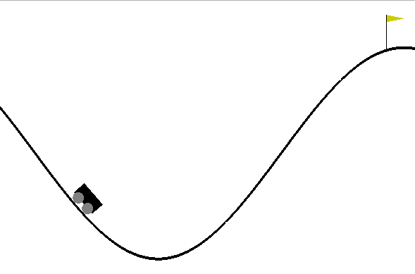
Figure: The mountain car simulation from the Open AI gym.

The goal is to define a sequence of actions (push the car right or left with certain intensity) to make the car reach the flag after a number \(T\) of time steps.

At each time step \(t\), the car is characterized by a vector \(\mathbf{ x}_{t} = (p_t,v_t)\) of states which are respectively the the position and velocity of the car at time \(t\). For a sequence of states (an episode), the dynamics of the car is given by

\[ \mathbf{ x}_{t+1} = f(\mathbf{ x}_{t},\textbf{u}_{t}) \]

where \(\textbf{u}_{t}\) is the value of an action force, which in this example corresponds to push car to the left (negative value) or to the right (positive value). The actions across a full episode are represented in a policy \(\textbf{u}_{t} = \pi(\mathbf{ x}_{t},\theta)\) that acts according to the current state of the car and some parameters \(\theta\). In the following examples we will assume that the policy is linear which allows us to write \(\pi(\mathbf{ x}_{t},\theta)\) as

Mountain Car Set Up

To run the mountain car example we need to install a python file that we’ll download.

import urllib.request

urllib.request.urlretrieve('https://raw.githubusercontent.com/lawrennd/talks/gh-pages/mountain_car.py','mountain_car.py')

And to render the environment, the pyglet library.

%pip install pyglet

\[ \pi(\mathbf{ x},\theta)= \theta_0 + \theta_p p + \theta_vv. \] For \(t=1,\dots,T\) now given some initial state \(\mathbf{ x}_{0}\) and some some values of each \(\textbf{u}_{t}\), we can simulate the full dynamics of the car for a full episode using Gym. The values of \(\textbf{u}_{t}\) are fully determined by the parameters of the linear controller.

After each episode of length \(T\) is complete, a reward function \(R_{T}(\theta)\) is computed. In the mountain car example, the reward is computed as 100 for reaching the target of the hill on the right hand side, minus the squared sum of actions (a real negative to push to the left and a real positive to push to the right) from start to goal. Note that our reward depends on \(\theta\) as we make it dependent on the parameters of the linear controller.

Emulate the Mountain Car

%pip install gym

import gym

env = gym.make('MountainCarContinuous-v0')

Our goal in this section is to find the parameters \(\theta\) of the linear controller such that

\[ \theta^* = arg \max_{\theta} R_T(\theta). \]

In this section, we directly use Bayesian optimization to solve this problem. We will use EmuKit so we first define the objective function.

import mountain_car as mc
import numpy as np

For each set of parameter values of the linear controller we can run an episode of the simulator (that we fix to have a horizon of \(T=500\)) to generate the reward. Using as input the parameters of the controller and as outputs the rewards we can build a Gaussian process emulator of the reward.

We start defining the input space, which is three-dimensional:

from emukit.core import ContinuousParameter, ParameterSpace

position_domain = [-1.2, +1]
velocity_domain = [-1/0.07, +1/0.07]
constant_domain = [-1, +1]

space = ParameterSpace(
          [ContinuousParameter('position_parameter', *position_domain), 
           ContinuousParameter('velocity_parameter', *velocity_domain),
           ContinuousParameter('constant', *constant_domain)])

To initalize the model we start sampling some initial points for the linear controller randomly.

from emukit.core.initial_designs import RandomDesign

design = RandomDesign(space)
n_initial_points = 25
initial_design = design.get_samples(n_initial_points)

Now run the simulation 25 times across our initial design.

y = target_function(initial_design)

Before we start any optimization, lets have a look to the behaviour of the car with the first of these initial points that we have selected randomly.

import numpy as np

This won’t render in Google colab, but should work in a regular Jupyter notebook if pyglet is installed. Details on rendering in colab are given in answer to this stackoverflow question https://stackoverflow.com/questions/50107530/how-to-render-openai-gym-in-google-colab.

random_controller = initial_design[0,:]
_, _, _, frames = mc.run_simulation(env, np.atleast_2d(random_controller), render=True)
anim=mc.animate_frames(frames, 'Random linear controller')

Figure: Random linear controller for the Mountain car. It fails to move the car to the top of the mountain.

As we can see the random linear controller does not manage to push the car to the top of the mountain. Now, let’s optimize the regret using Bayesian optimization and the emulator for the reward. We try 50 new parameters chosen by the expected improvement acquisition function.

First, we initizialize a Gaussian process emulator.

import GPy

kern = GPy.kern.RBF(3)
model_gpy = GPy.models.GPRegression(initial_design, y, kern, noise_var=1e-10)

from emukit.model_wrappers.gpy_model_wrappers import GPyModelWrapper

model_emukit = GPyModelWrapper(model_gpy, n_restarts=5)
model_emukit.optimize()

In Bayesian optimization an acquisition function is used to balance exploration and exploitation to evaluate new locations close to the optimum of the objective. In this notebook we select the expected improvement (EI). For further details have a look at the review paper of Shahriari et al. (2016).

from emukit.bayesian_optimization.acquisitions import ExpectedImprovement

acquisition = ExpectedImprovement(model_emukit)

from emukit.bayesian_optimization.loops.bayesian_optimization_loop import BayesianOptimizationLoop

bo = BayesianOptimizationLoop(space, model_emukit, acquisition=acquisition)
bo.run_loop(target_function, 50)
results= bo.get_results()

Now we visualize the result for the best controller that we have found with Bayesian optimization.

_, _, _, frames = mc.run_simulation(env, np.atleast_2d(results.minimum_location), render=True)
anim=mc.animate_frames(frames, 'Best controller after 50 iterations of Bayesian optimization')

Figure: Mountain car simulator trained using Bayesian optimization and the simulator of the dynamics. Fifty iterations of Bayesian optimization are used to optimize the controler.

The car can now make it to the top of the mountain! Emulating the reward function and using expected improvement acquisition helped us to find a linear controller that solves the problem.

Data Efficient Emulation

In the previous section we solved the mountain car problem by directly emulating the reward but no considerations about the dynamics \[ \mathbf{ x}_{t+1} =g(\mathbf{ x}_{t},\textbf{u}_{t}) \] of the system were made.

We ran the simulator 25 times in the initial design, and 50 times in our Bayesian optimization loop. That required us to call the dynamics simulation \(500\times 75 =37,500\) times, because each simulation of the car used 500 steps. In this section we will show how it is possible to reduce this number by building an emulator for \(g(\cdot)\) that can later be used to directly optimize the control.

The inputs of the model for the dynamics are the velocity, the position and the value of the control so create this space accordingly.

import gym

env = gym.make('MountainCarContinuous-v0')

from emukit.core import ContinuousParameter, ParameterSpace

position_dynamics_domain = [-1.2, +0.6]
velocity_dynamics_domain = [-0.07, +0.07]
action_dynamics_domain = [-1, +1]

space_dynamics = ParameterSpace(
          [ContinuousParameter('position_dynamics_parameter', *position_dynamics_domain), 
           ContinuousParameter('velocity_dynamics_parameter', *velocity_dynamics_domain),
           ContinuousParameter('action_dynamics_parameter', *action_dynamics_domain)])

Next, we sample some input parameters and use the simulator to compute the outputs. Note that in this case we are not running the full episodes, we are just using the simulator to compute \(\mathbf{ x}_{t+1}\) given \(\mathbf{ x}_{t}\) and \(\textbf{u}_{t}\).

from emukit.core.initial_designs import RandomDesign

design_dynamics = RandomDesign(space_dynamics)
n_initial_points = 500
initial_design_dynamics = design_dynamics.get_samples(n_initial_points)

import numpy as np
import mountain_car as mc

### --- Simulation of the (normalized) outputs
y_dynamics = np.zeros((initial_design_dynamics.shape[0], 2))
for i in range(initial_design_dynamics.shape[0]):
    y_dynamics[i, :] = mc.simulation(initial_design_dynamics[i, :])

# Normalize the data from the simulation
y_dynamics_normalisation = np.std(y_dynamics, axis=0)
y_dynamics_normalised = y_dynamics/y_dynamics_normalisation

The outputs are the velocity and the position. Our model will capture the change in position and velocity on time. That is, we will model

\[ \Delta v_{t+1} = v_{t+1} - v_{t} \]

\[ \Delta x_{t+1} = p_{t+1} - p_{t} \]

with Gaussian processes with prior mean \(v_{t}\) and \(p_{t}\) respectively. As a covariance function, we use Matern52. We need therefore two models to capture the full dynamics of the system.

import GPy

kern_position = GPy.kern.Matern52(3)
position_model_gpy = GPy.models.GPRegression(initial_design_dynamics, y_dynamics[:, 0:1], kern_position, noise_var=1e-10)

kern_velocity = GPy.kern.Matern52(3)
velocity_model_gpy = GPy.models.GPRegression(initial_design_dynamics, y_dynamics[:, 1:2], kern_velocity, noise_var=1e-10)

from emukit.model_wrappers.gpy_model_wrappers import GPyModelWrapper

position_model_emukit = GPyModelWrapper(position_model_gpy, n_restarts=5)
velocity_model_emukit = GPyModelWrapper(velocity_model_gpy, n_restarts=5)

In general, we might use much smarter strategies to design our emulation of the simulator. For example, we could use the variance of the predictive distributions of the models to collect points using uncertainty sampling, which will give us a better coverage of the space. For simplicity, we move ahead with the 500 randomly selected points.

Now that we have a data set, we can update the emulators for the location and the velocity.

position_model_emukit.optimize()
velocity_model_emukit.optimize()

We can now have a look to how the emulator and the simulator match. First, we show a contour plot of the car acceleration for each pair of can position and velocity. You can use the bar bellow to play with the values of the controller to compare the emulator and the simulator.

We can see how the emulator is doing a fairly good job approximating the simulator. On the edges, however, it struggles to captures the dynamics of the simulator.

Given some input parameters of the linear controlling, how do the dynamics of the emulator and simulator match? In the following figure we show the position and velocity of the car for the 500 time-steps of an episode in which the parameters of the linear controller have been fixed beforehand. The value of the input control is also shown.

# change the values of the linear controller to observe the trajectories.
controller_gains = np.atleast_2d([0, .6, 1])  

Figure: Comparison between the mountain car simulator and the emulator.

We now make explicit use of the emulator, using it to replace the simulator and optimize the linear controller. Note that in this optimization, we don’t need to query the simulator anymore as we can reproduce the full dynamics of an episode using the emulator. For illustrative purposes, in this example we fix the initial location of the car.

We define the objective reward function in terms of the simulator.

### --- Optimize control parameters with emulator
car_initial_location = np.asarray([-0.58912799, 0])

And as before, we use Bayesian optimization to find the best possible linear controller.

The design space is the three continuous variables that make up the linear controller.

position_domain = [-1.2, +1]
velocity_domain = [-1/0.07, +1/0.07]
constant_domain = [-1, +1]

space = ParameterSpace(
          [ContinuousParameter('position_parameter', *position_domain), 
           ContinuousParameter('velocity_parameter', *velocity_domain),
           ContinuousParameter('constant', *constant_domain)])

from emukit.core.initial_designs import RandomDesign

design = RandomDesign(space)
n_initial_points = 25
initial_design = design.get_samples(n_initial_points)

Now run the simulation 25 times across our initial design.

y = target_function_emulator(initial_design)

Now we set up the surrogate model for the Bayesian optimization loop.

import GPy

kern = GPy.kern.RBF(3)
model_dynamics_emulated_gpy = GPy.models.GPRegression(initial_design, y, kern, noise_var=1e-10)

from emukit.model_wrappers.gpy_model_wrappers import GPyModelWrapper

model_dynamics_emulated_emukit = GPyModelWrapper(model_dynamics_emulated_gpy, n_restarts=5)
model_dynamics_emulated_emukit.optimize()

We set the acquisition function to be expected improvement.

from emukit.bayesian_optimization.acquisitions import ExpectedImprovement

acquisition = ExpectedImprovement(model_emukit)

And we set up the main loop for the Bayesian optimization.

from emukit.bayesian_optimization.loops.bayesian_optimization_loop import BayesianOptimizationLoop

bo = BayesianOptimizationLoop(space, model_dynamics_emulated_emukit, acquisition=acquisition)
bo.run_loop(target_function_emulator, 50)
results = bo.get_results()

_, _, _, frames = mc.run_simulation(env, np.atleast_2d(results.minimum_location), render=True)
anim=mc.animate_frames(frames, 'Best controller using the emulator of the dynamics')

from IPython.core.display import HTML

Figure: Mountain car controller learnt through emulation. Here 500 calls to the simulator are used to fit the controller rather than 37,500 calls to the simulator required in the standard learning.

And the problem is again solved, but in this case, we have replaced the simulator of the car dynamics by a Gaussian process emulator that we learned by calling the dynamics simulator only 500 times. Compared to the 37,500 calls that we needed when applying Bayesian optimization directly on the simulator this is a significant improvement. Of course, in practice the car dynamics are very simple for this example.

Mountain Car: Multi-Fidelity Emulation

In some scenarios we have simulators of the same environment that have different fidelities, that is that reflect with different level of accuracy the dynamics of the real world. Running simulations of the different fidelities also have a different cost: high-fidelity simulations are typically more expensive the low-fidelity. If we have access to these simulators, we can combine high and low-fidelity simulations under the same model.

So, let’s assume that we have two simulators of the mountain car dynamics, one of high fidelity (the one we have used) and another one of low fidelity. The traditional approach to this form of multi-fidelity emulation is to assume that \[ f_i\left(\mathbf{ x}\right) = \rho f_{i-1}\left(\mathbf{ x}\right) + \delta_i\left(\mathbf{ x}\right), \] where \(f_{i-1}\left(\mathbf{ x}\right)\) is a low-fidelity simulation of the problem of interest and \(f_i\left(\mathbf{ x}\right)\) is a higher fidelity simulation. The function \(\delta_i\left(\mathbf{ x}\right)\) represents the difference between the lower and higher fidelity simulation, which is considered additive. The additive form of this covariance means that if \(f_{0}\left(\mathbf{ x}\right)\) and \(\left\{\delta_i\left(\mathbf{ x}\right)\right\}_{i=1}^m\) are all Gaussian processes, then the process over all fidelities of simulation will be a joint Gaussian process.

But with deep Gaussian processes we can consider the form \[ f_i\left(\mathbf{ x}\right) = g_{i}\left(f_{i-1}\left(\mathbf{ x}\right)\right) + \delta_i\left(\mathbf{ x}\right), \] where the low fidelity representation is nonlinearly transformed by \(g(\cdot)\) before use in the process. This is the approach taken in Perdikaris et al. (2017). But once we accept that these models can be composed, a highly flexible framework can emerge. A key point is that the data enters the model at different levels and represents different aspects. For example, these correspond to the two fidelities of the mountain car simulator.

We start by sampling both at 250 random input locations.

import gym

env = gym.make('MountainCarContinuous-v0')

from emukit.core import ContinuousParameter, ParameterSpace

position_dynamics_domain = [-1.2, +0.6]
velocity_dynamics_domain = [-0.07, +0.07]
action_dynamics_domain = [-1, +1]

space_dynamics = ParameterSpace(
          [ContinuousParameter('position_dynamics_parameter', *position_dynamics_domain), 
           ContinuousParameter('velocity_dynamics_parameter', *velocity_dynamics_domain),
           ContinuousParameter('action_dynamics_parameter', *action_dynamics_domain)])

Next, we evaluate the high and low fidelity simualtors at those locations.

import numpy as np
import mountain_car as mc

n_points = 250
d_position_hf = np.zeros((n_points, 1))
d_velocity_hf = np.zeros((n_points, 1))
d_position_lf = np.zeros((n_points, 1))
d_velocity_lf = np.zeros((n_points, 1))

# --- Collect high fidelity points
for i in range(0, n_points):
    d_position_hf[i], d_velocity_hf[i] = mc.simulation(x_random[i, :])

# --- Collect low fidelity points  
for i in range(0, n_points):
    d_position_lf[i], d_velocity_lf[i] = mc.low_cost_simulation(x_random[i, :])

Building the Multifidelity Emulation

It is time to build the multi-fidelity model for both the position and the velocity.

As we did in the previous section we use the emulator to optimize the simulator. In this case we use the high fidelity output of the emulator.

First we optimize the controller parameters

And we optimize using Bayesian optimzation.

from emukit.core import ContinuousParameter, ParameterSpace

position_domain = [-1.2, +1]
velocity_domain = [-1/0.07, +1/0.07]
constant_domain = [-1, +1]

space = ParameterSpace(
          [ContinuousParameter('position_parameter', *position_domain), 
           ContinuousParameter('velocity_parameter', *velocity_domain),
           ContinuousParameter('constant', *constant_domain)])

from emukit.core.initial_designs import RandomDesign

design = RandomDesign(space)
n_initial_points = 25
initial_design = design.get_samples(n_initial_points)

n_initial_points = 25 random_design = RandomDesign(design_space) initial_design = random_design.get_samples(n_initial_points) acquisition = GPyOpt.acquisitions.AcquisitionEI(model, design_space, optimizer=aquisition_optimizer) evaluator = GPyOpt.core.evaluators.Sequential(acquisition)}

bo_multifidelity = GPyOpt.methods.ModularBayesianOptimization(model, design_space, objective_multifidelity, acquisition, evaluator, initial_design)
bo_multifidelity.run_optimization(max_iter=50)

_, _, _, frames = mc.run_simulation(env, np.atleast_2d(bo_multifidelity.x_opt), render=True)
anim=mc.animate_frames(frames, 'Best controller with multi-fidelity emulator')

Best Controller with Multi-Fidelity Emulator

Figure: Mountain car learnt with multi-fidelity model. Here 250 observations of the high fidelity simulator and 250 observations of the low fidelity simulator are used to learn the controller.

And problem solved! We see how the problem is also solved with 250 observations of the high fidelity simulator and 250 of the low fidelity simulator.

Emukit Playground

Emukit playground is a software toolkit for exploring the use of statistical emulation as a tool. It was built by Leah Hirst, during her software engineering internship at Amazon and supervised by Cliff McCollum.

Figure: Emukit playground is a tutorial for understanding the simulation/emulation relationship. https://amzn.github.io/emukit-playground/

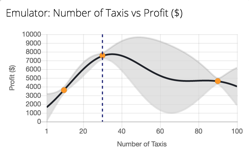
Figure: Tutorial on Bayesian optimization of the number of taxis deployed from Emukit playground. https://amzn.github.io/emukit-playground/#!/learn/bayesian_optimization

You can explore Bayesian optimization of a taxi simulation.

Emukit

The Emukit software we will be using across the next part of this module is a python software library that facilitates emulation of systems. The software’s origins go back to work done by Javier Gonzalez as part of his post-doctoral project at the University of Sheffield. Javier led the design and build of a Bayesian optimization software. The package GPyOpt worked with the SheffieldML software GPy for performing Bayesian optimization.

GPyOpt has a modular design that allows the user to provide their own surrogate models, the package is build with GPy as a surrogate model in mind, but other surrogate models can also be wrapped and integrated.

However, GPyOpt doesn’t allow the full flexibility of surrogate modelling for domains like experimental design, sensitivity analysis etc.

Emukit was designed and built for a more general approach. The software is MIT licensed and its design and implementation was led by Javier Gonzalez and Andrei Paleyes at Amazon. Building on the experience of GPyOpt, the aim with Emukit was to use the modularisation ideas embedded in GPyOpt, but to extend them beyond the modularisation of the surrogate models to modularisation of the acquisition function.

Figure: The Emukit software is a set of software tools for emulation and surrogate modeling. https://emukit.github.io/emukit/

%pip install gpy

%pip install pyDOE

%pip install emukit

The software was initially built by the team in Amazon. As well as Javier Gonzalez (ML side) and Andrei Paleyes (Software Engineering) included Mark Pullin, Maren Mahsereci, Alex Gessner, Aaron Klein, Henry Moss, David-Elias Künstle as well as management input from Cliff McCollum and myself.

{For monitoring systems in production, emulation needn’t just be about simulator models. What we envisage, is that even data driven models could be emulated. This is important for understanding system behaviour, how the different components are interconnected. This drives the notion of the information dynamics of the machine learning system. What is the effect of one particular intervention in the wider system? One way of answering this is through emulation. But it requires that our machine learning models (and our simulators) are deployed in an environment where emulation can be automatically deployed. The resulting system would allow us to monitor the downstream effects of indivdiual decision making on the wider system.

blog post on New Directions in Kernels and Gaussian Processes.

Deep Gaussian Processes

One challenge is developing flexible enough models to perform the emulation that also propagate uncertainty through the model. One candidate set of models for this challenge is deep Gaussian processes (DGPs). For the remainder of these notes we introduce the theory behind DGPs.

While there are some difficulties in algorithmically implementing these algorithms at scale, they are mathematically far simpler than the equivalent neural network models, and perhaps as a result offer greater promise for theoretical understanding of deep learning (see e.g. Dunlop et al., n.d.).

Bottleneck Layers in Deep Neural Networks

Figure: Inserting the bottleneck layers introduces a new set of variables.

Including the low rank decomposition of \(\mathbf{W}\) in the neural network, we obtain a new mathematical form. Effectively, we are adding additional latent layers, \(\mathbf{ z}\), in between each of the existing hidden layers. In a neural network these are sometimes known as bottleneck layers. The network can now be written mathematically as \[ \begin{align} \mathbf{ z}_{1} &= \mathbf{V}^\top_1 \mathbf{ x}\\ \mathbf{ h}_{1} &= \phi\left(\mathbf{U}_1 \mathbf{ z}_{1}\right)\\ \mathbf{ z}_{2} &= \mathbf{V}^\top_2 \mathbf{ h}_{1}\\ \mathbf{ h}_{2} &= \phi\left(\mathbf{U}_2 \mathbf{ z}_{2}\right)\\ \mathbf{ z}_{3} &= \mathbf{V}^\top_3 \mathbf{ h}_{2}\\ \mathbf{ h}_{3} &= \phi\left(\mathbf{U}_3 \mathbf{ z}_{3}\right)\\ \mathbf{ y}&= \mathbf{ w}_4^\top\mathbf{ h}_{3}. \end{align} \]

\[ \begin{align} \mathbf{ z}_{1} &= \mathbf{V}^\top_1 \mathbf{ x}\\ \mathbf{ z}_{2} &= \mathbf{V}^\top_2 \phi\left(\mathbf{U}_1 \mathbf{ z}_{1}\right)\\ \mathbf{ z}_{3} &= \mathbf{V}^\top_3 \phi\left(\mathbf{U}_2 \mathbf{ z}_{2}\right)\\ \mathbf{ y}&= \mathbf{ w}_4 ^\top \mathbf{ z}_{3} \end{align} \]

Cascade of Gaussian Processes

Now if we replace each of these neural networks with a Gaussian process. This is equivalent to taking the limit as the width of each layer goes to infinity, while appropriately scaling down the outputs.

\[ \begin{align} \mathbf{ z}_{1} &= \mathbf{ f}_1\left(\mathbf{ x}\right)\\ \mathbf{ z}_{2} &= \mathbf{ f}_2\left(\mathbf{ z}_{1}\right)\\ \mathbf{ z}_{3} &= \mathbf{ f}_3\left(\mathbf{ z}_{2}\right)\\ \mathbf{ y}&= \mathbf{ f}_4\left(\mathbf{ z}_{3}\right) \end{align} \]

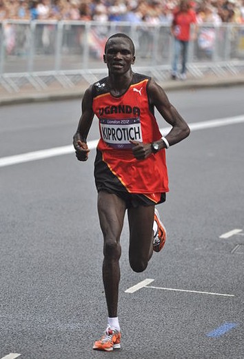
Olympic Marathon Data

Gold medal times for Olympic Marathon since 1896. Marathons before 1924 didn’t have a standardised distance. Present results using pace per km. In 1904 Marathon was badly organised leading to very slow times.

Image from Wikimedia Commons http://bit.ly/16kMKHQ

The first thing we will do is load a standard data set for regression modelling. The data consists of the pace of Olympic Gold Medal Marathon winners for the Olympics from 1896 to present. First we load in the data and plot.

import numpy as np
import pods

data = pods.datasets.olympic_marathon_men()
x = data['X']
y = data['Y']

offset = y.mean()
scale = np.sqrt(y.var())

Figure: Olympic marathon pace times since 1896.

Things to notice about the data include the outlier in 1904, in this year, the olympics was in St Louis, USA. Organizational problems and challenges with dust kicked up by the cars following the race meant that participants got lost, and only very few participants completed.

More recent years see more consistently quick marathons.

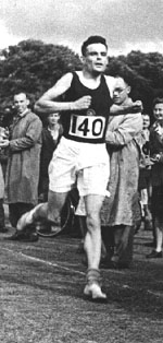
Alan Turing

Figure: Alan Turing, in 1946 he was only 11 minutes slower than the winner of the 1948 games. Would he have won a hypothetical games held in 1946? Source: Alan Turing Internet Scrapbook.

If we had to summarise the objectives of machine learning in one word, a very good candidate for that word would be generalization. What is generalization? From a human perspective it might be summarised as the ability to take lessons learned in one domain and apply them to another domain. If we accept the definition given in the first session for machine learning, \[ \text{data} + \text{model} \stackrel{\text{compute}}{\rightarrow} \text{prediction} \] then we see that without a model we can’t generalise: we only have data. Data is fine for answering very specific questions, like “Who won the Olympic Marathon in 2012?” because we have that answer stored, however, we are not given the answer to many other questions. For example, Alan Turing was a formidable marathon runner, in 1946 he ran a time 2 hours 46 minutes (just under four minutes per kilometer, faster than I and most of the other Endcliffe Park Run runners can do 5 km). What is the probability he would have won an Olympics if one had been held in 1946?

To answer this question we need to generalize, but before we formalize the concept of generalization let’s introduce some formal representation of what it means to generalize in machine learning.

Gaussian Process Fit

Our first objective will be to perform a Gaussian process fit to the data, we’ll do this using the GPy software.

import GPy

m_full = GPy.models.GPRegression(x,yhat)
_ = m_full.optimize() # Optimize parameters of covariance function

The first command sets up the model, then m_full.optimize() optimizes the parameters of the covariance function and the noise level of the model. Once the fit is complete, we’ll try creating some test points, and computing the output of the GP model in terms of the mean and standard deviation of the posterior functions between 1870 and 2030. We plot the mean function and the standard deviation at 200 locations. We can obtain the predictions using y_mean, y_var = m_full.predict(xt)

xt = np.linspace(1870,2030,200)[:,np.newaxis]
yt_mean, yt_var = m_full.predict(xt)
yt_sd=np.sqrt(yt_var)

Now we plot the results using the helper function in teaching_plots.

Figure: Gaussian process fit to the Olympic Marathon data. The error bars are too large, perhaps due to the outlier from 1904.

Fit Quality

In the fit we see that the error bars (coming mainly from the noise variance) are quite large. This is likely due to the outlier point in 1904, ignoring that point we can see that a tighter fit is obtained. To see this make a version of the model, m_clean, where that point is removed.

x_clean=np.vstack((x[0:2, :], x[3:, :]))
y_clean=np.vstack((y[0:2, :], y[3:, :]))

m_clean = GPy.models.GPRegression(x_clean,y_clean)
_ = m_clean.optimize()

Deep GP Fit

Let’s see if a deep Gaussian process can help here. We will construct a deep Gaussian process with one hidden layer (i.e. one Gaussian process feeding into another).

Build a Deep GP with an additional hidden layer (one dimensional) to fit the model.

import GPy
import deepgp

hidden = 1
m = deepgp.DeepGP([y.shape[1],hidden,x.shape[1]],Y=yhat, X=x, inits=['PCA','PCA'], 
                  kernels=[GPy.kern.RBF(hidden,ARD=True),
                           GPy.kern.RBF(x.shape[1],ARD=True)], # the kernels for each layer
                  num_inducing=50, back_constraint=False)

import deepgp

# Call the initalization
m.initialize()

Now optimize the model.

for layer in m.layers:
    layer.likelihood.variance.constrain_positive(warning=False)
m.optimize(messages=True,max_iters=10000)

m.staged_optimize(messages=(True,True,True))

Olympic Marathon Data Deep GP

Figure: Deep GP fit to the Olympic marathon data. Error bars now change as the prediction evolves.

Olympic Marathon Data Deep GP

Figure: Point samples run through the deep Gaussian process show the distribution of output locations.

Fitted GP for each layer

Now we explore the GPs the model has used to fit each layer. First of all, we look at the hidden layer.

Figure: The mapping from input to the latent layer is broadly, with some flattening as time goes on. Variance is high across the input range.

Figure: The mapping from the latent layer to the output layer.

Olympic Marathon Pinball Plot

Figure: A pinball plot shows the movement of the ‘ball’ as it passes through each layer of the Gaussian processes. Mean directions of movement are shown by lines. Shading gives one standard deviation of movement position. At each layer, the uncertainty is reset. The overal uncertainty is the cumulative uncertainty from all the layers. There is some grouping of later points towards the right in the first layer, which also injects a large amount of uncertainty. Due to flattening of the curve in the second layer towards the right the uncertainty is reduced in final output.

The pinball plot shows the flow of any input ball through the deep Gaussian process. In a pinball plot a series of vertical parallel lines would indicate a purely linear function. For the olypmic marathon data we can see the first layer begins to shift from input towards the right. Note it also does so with some uncertainty (indicated by the shaded backgrounds). The second layer has less uncertainty, but bunches the inputs more strongly to the right. This input layer of uncertainty, followed by a layer that pushes inputs to the right is what gives the heteroschedastic noise.

MXFusion: Modular Probabilistic Programming on MXNet

One challenge for practitioners in Gaussian processes, is flexible software that allows the construction of the relevant GP modle. With this in mind, the Amazon Cambridge team has developed MXFusion. It is a modular probabilistic programming language focussed on efficient implementation of hybrid GP-neural network models, but with additional probabilistic programming capabilities.

Figure: MXFusion is a probabilistic programming language targeted specifically at Gaussian process models and combining them with probaiblistic neural network. It is available through the MIT license and we welcome contributions throguh the Github repository https://github.com/amzn/MXFusion.

We developed the framework for greater ease of transitioning models from ‘science’ to ‘production,’ our aim was to have code that could be created by scientists, but deployed in our systems through solutions such as AWS SageMaker.

\ericMeissner{15%}\zhenwenDai{15%}

Work by Eric Meissner and Zhenwen Dai. Probabilistic programming. Available on Github

Figure: The MXFusion software.

Conclusion

Machine learning models are deployed as components in an interacting system to achieve modern AI. Some of those components are inspired by a mechanistic understanding of the world around us (e.g. economic or physical understanding).

Meta modelling involves fiting machine learning models to existing systems to improve speed and interpretability.

Deep Gaussian processes are a flexible approach to meta modelling, which provide the necessary uncertainty estimates and the potential for being more mathematically tractable.

Thanks!

For more information on these subjects and more you might want to check the following resources.

• twitter: @lawrennd
• podcast: The Talking Machines
• newspaper: Guardian Profile Page
• blog: http://inverseprobability.com

References