Abstract

A vital perspective is missing from the discussions we’re having about Artificial Intelligence: what does it mean for our identity?

Our fascination with AI stems from the perceived uniqueness of human intelligence. We believe it’s what differentiates us. Fears of AI not only concern how it invades our digital lives, but also the implied threat of an intelligence that displaces us from our position at the centre of the world.

Atomism, proposed by Democritus, suggested it was impossible to continue dividing matter down into ever smaller components: eventually we reach a point where a cut cannot be made (the Greek for uncuttable is ‘atom’). In the same way, by slicing away at the facets of human intelligence that can be replaced by machines, AI uncovers what is left: an indivisible core that is the essence of humanity.

By contrasting our own (evolved, locked-in, embodied) intelligence with the capabilities of machine intelligence through history, The Atomic Human reveals the technical origins, capabilities and limitations of AI systems, and how they should be wielded. Not just by the experts, but ordinary people. Either AI is a tool for us, or we become a tool of AI. Understanding this will enable us to choose the future we want.

This talk is based on Neil’s forthcoming book to be published with Allen Lane in June 2024. Machine learning solutions, in particular those based on deep learning methods, form an underpinning of the current revolution in “artificial intelligence” that has dominated popular press headlines and is having a significant influence on the wider tech agenda.

In this talk I will give an overview of where we are now with machine learning solutions, and what challenges we face both in the near and far future. These include practical application of existing algorithms in the face of the need to explain decision making, mechanisms for improving the quality and availability of data, dealing with large unstructured datasets.

Henry Ford’s Faster Horse

Figure: A 1925 Ford Model T built at Henry Ford’s Highland Park Plant in Dearborn, Michigan. This example now resides in Australia, owned by the founder of FordModelT.net. From https://commons.wikimedia.org/wiki/File:1925_Ford_Model_T_touring.jpg

It’s said that Henry Ford’s customers wanted a “a faster horse”. If Henry Ford was selling us artificial intelligence today, what would the customer call for, “a smarter human”? That’s certainly the picture of machine intelligence we find in science fiction narratives, but the reality of what we’ve developed is much more mundane.

Car engines produce prodigious power from petrol. Machine intelligences deliver decisions derived from data. In both cases the scale of consumption enables a speed of operation that is far beyond the capabilities of their natural counterparts. Unfettered energy consumption has consequences in the form of climate change. Does unbridled data consumption also have consequences for us?

If we devolve decision making to machines, we depend on those machines to accommodate our needs. If we don’t understand how those machines operate, we lose control over our destiny. Our mistake has been to see machine intelligence as a reflection of our intelligence. We cannot understand the smarter human without understanding the human. To understand the machine, we need to better understand ourselves.

The Diving Bell and the Butterfly

Figure: The Diving Bell and the Buttefly is the autobiography of Jean Dominique Bauby.

The Diving Bell and the Butterfly is the autobiography of Jean Dominique Bauby. Jean Dominique, the editor of French Elle magazine, suffered a major stroke at the age of 43 in 1995. The stroke paralyzed him and rendered him speechless. He was only able to blink his left eyelid, he became a sufferer of locked in syndrome.

E S A R I N T U L
O M D P C F B V
H G J Q Z Y X K W

Figure: The ordering of the letters that Bauby used for writing his autobiography.

How could he do that? Well, first, they set up a mechanism where he could scan across letters and blink at the letter he wanted to use. In this way, he was able to write each letter.

It took him 10 months of four hours a day to write the book. Each word took two minutes to write.

Imagine doing all that thinking, but so little speaking, having all those thoughts and so little ability to communicate.

The idea behind this talk is that we are all in that situation. While not as extreme as for Bauby, we all have somewhat of a locked in intelligence.

Figure: Jean Dominique Bauby was the Editor in Chief of the French Elle Magazine, he suffered a stroke that destroyed his brainstem, leaving him only capable of moving one eye. Jean Dominique became a victim of locked in syndrome.

Incredibly, Jean Dominique wrote his book after he became locked in. It took him 10 months of four hours a day to write the book. Each word took two minutes to write.

The idea behind embodiment factors is that we are all in that situation. While not as extreme as for Bauby, we all have somewhat of a locked in intelligence.

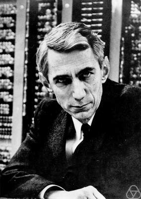
Figure: Claude Shannon developed information theory which allows us to quantify how much Bauby can communicate. This allows us to compare how locked in he is to us.

The Atomic Human

Figure: The Atomic Eye, by slicing away aspects of the human that we used to believe to be unique to us, but are now the preserve of the machine, we learn something about what it means to be human.

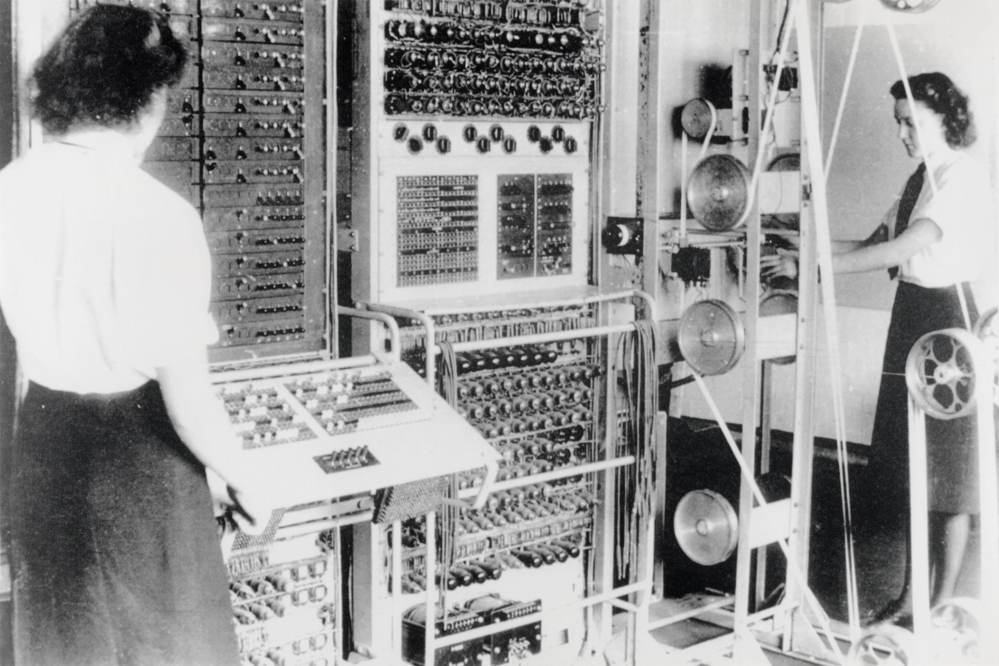
Figure: A Colossus Mark 2 codebreaking computer being operated by Dorothy Du Boisson (left) and Elsie Booker (right). Colossus was designed by Tommy Flowers, but programmed and operated by groups of Wrens based at Bletchley Park.

Embodiment Factors

bits/min	billions	2,000
billion calculations/s	~100	a billion
embodiment	20 minutes	5 billion years

Figure: Embodiment factors are the ratio between our ability to compute and our ability to communicate. Relative to the machine we are also locked in. In the table we represent embodiment as the length of time it would take to communicate one second’s worth of computation. For computers it is a matter of minutes, but for a human, it is a matter of thousands of millions of years. See also “Living Together: Mind and Machine Intelligence” Lawrence (2017)

There is a fundamental limit placed on our intelligence based on our ability to communicate. Claude Shannon founded the field of information theory. The clever part of this theory is it allows us to separate our measurement of information from what the information pertains to.¹

Shannon measured information in bits. One bit of information is the amount of information I pass to you when I give you the result of a coin toss. Shannon was also interested in the amount of information in the English language. He estimated that on average a word in the English language contains 12 bits of information.

Given typical speaking rates, that gives us an estimate of our ability to communicate of around 100 bits per second (Reed and Durlach, 1998). Computers on the other hand can communicate much more rapidly. Current wired network speeds are around a billion bits per second, ten million times faster.

When it comes to compute though, our best estimates indicate our computers are slower. A typical modern computer can process make around 100 billion floating-point operations per second, each floating-point operation involves a 64 bit number. So the computer is processing around 6,400 billion bits per second.

It’s difficult to get similar estimates for humans, but by some estimates the amount of compute we would require to simulate a human brain is equivalent to that in the UK’s fastest computer (Ananthanarayanan et al., 2009), the MET office machine in Exeter, which in 2018 ranked as the 11th fastest computer in the world. That machine simulates the world’s weather each morning, and then simulates the world’s climate in the afternoon. It is a 16-petaflop machine, processing around 1,000 trillion bits per second.

Bandwidth Constrained Conversations

Figure: Conversation relies on internal models of other individuals.

Figure: Misunderstanding of context and who we are talking to leads to arguments.

Embodiment factors imply that, in our communication between humans, what is not said is, perhaps, more important than what is said. To communicate with each other we need to have a model of who each of us are.

To aid this, in society, we are required to perform roles. Whether as a parent, a teacher, an employee or a boss. Each of these roles requires that we conform to certain standards of behaviour to facilitate communication between ourselves.

Control of self is vitally important to these communications.

The high availability of data available to humans undermines human-to-human communication channels by providing new routes to undermining our control of self.

The consequences between this mismatch of power and delivery are to be seen all around us. Because, just as driving an F1 car with bicycle wheels would be a fine art, so is the process of communication between humans.

If I have a thought and I wish to communicate it, I first need to have a model of what you think. I should think before I speak. When I speak, you may react. You have a model of who I am and what I was trying to say, and why I chose to say what I said. Now we begin this dance, where we are each trying to better understand each other and what we are saying. When it works, it is beautiful, but when mis-deployed, just like a badly driven F1 car, there is a horrible crash, an argument.

Sistine Chapel Ceiling

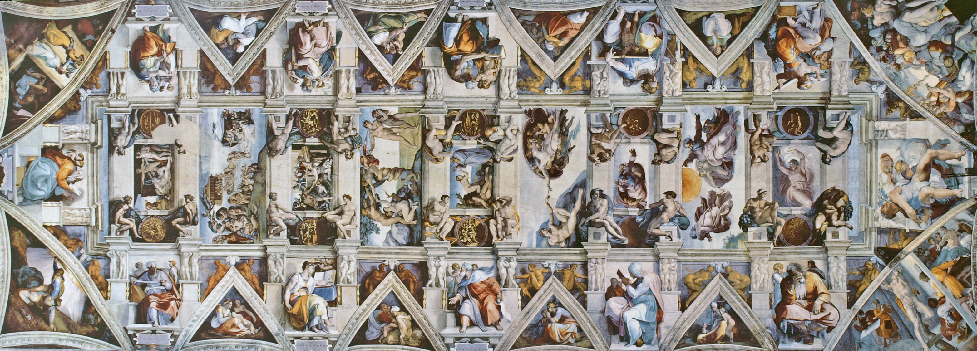
Figure: The ceiling of the Sistine Chapel.

Patrick Boyde’s talks on the Sistine Chapel focussed on both the structure of the chapel ceiling, describing the impression of height it was intended to give, as well as the significance and positioning of each of the panels and the meaning of the individual figures.

The Creation of Man

Figure: Photo of Detail of Creation of Man from the Sistine chapel ceiling.

One of the most famous panels is central in the ceiling, it’s the creation of man. Here, God in the guise of a pink-robed bearded man reaches out to a languid Adam.

The representation of God in this form seems typical of the time, because elsewhere in the Vatican Museums there are similar representations.

Figure: Photo detail of God.

https://commons.wikimedia.org/wiki/File:Michelangelo,_Creation_of_Adam_04.jpg

New Flow of Information

Classically the field of statistics focused on mediating the relationship between the machine and the human. Our limited bandwidth of communication means we tend to over-interpret the limited information that we are given, in the extreme we assign motives and desires to inanimate objects (a process known as anthropomorphizing). Much of mathematical statistics was developed to help temper this tendency and understand when we are valid in drawing conclusions from data.

Figure: The trinity of human, data, and computer, and highlights the modern phenomenon. The communication channel between computer and data now has an extremely high bandwidth. The channel between human and computer and the channel between data and human is narrow. New direction of information flow, information is reaching us mediated by the computer. The focus on classical statistics reflected the importance of the direct communication between human and data. The modern challenges of data science emerge when that relationship is being mediated by the machine.

Data science brings new challenges. In particular, there is a very large bandwidth connection between the machine and data. This means that our relationship with data is now commonly being mediated by the machine. Whether this is in the acquisition of new data, which now happens by happenstance rather than with purpose, or the interpretation of that data where we are increasingly relying on machines to summarize what the data contains. This is leading to the emerging field of data science, which must not only deal with the same challenges that mathematical statistics faced in tempering our tendency to over interpret data but must also deal with the possibility that the machine has either inadvertently or maliciously misrepresented the underlying data.

A Six Word Novel

Figure: Consider the six-word novel, apocryphally credited to Ernest Hemingway, “For sale: baby shoes, never worn”. To understand what that means to a human, you need a great deal of additional context. Context that is not directly accessible to a machine that has not got both the evolved and contextual understanding of our own condition to realize both the implication of the advert and what that implication means emotionally to the previous owner.

But this is a very different kind of intelligence than ours. A computer cannot understand the depth of the Ernest Hemingway’s apocryphal six-word novel: “For Sale, Baby Shoes, Never worn”, because it isn’t equipped with that ability to model the complexity of humanity that underlies that statement.

Revolution

Arguably the information revolution we are experiencing is unprecedented in history. But changes in the way we share information have a long history. Over 5,000 years ago in the city of Uruk, on the banks of the Euphrates, communities which relied on the water to irrigate their corps developed an approach to recording transactions in clay. Eventually the system of recording system became sophisticated enough that their oral histories could be recorded in the form of the first epic: Gilgamesh.

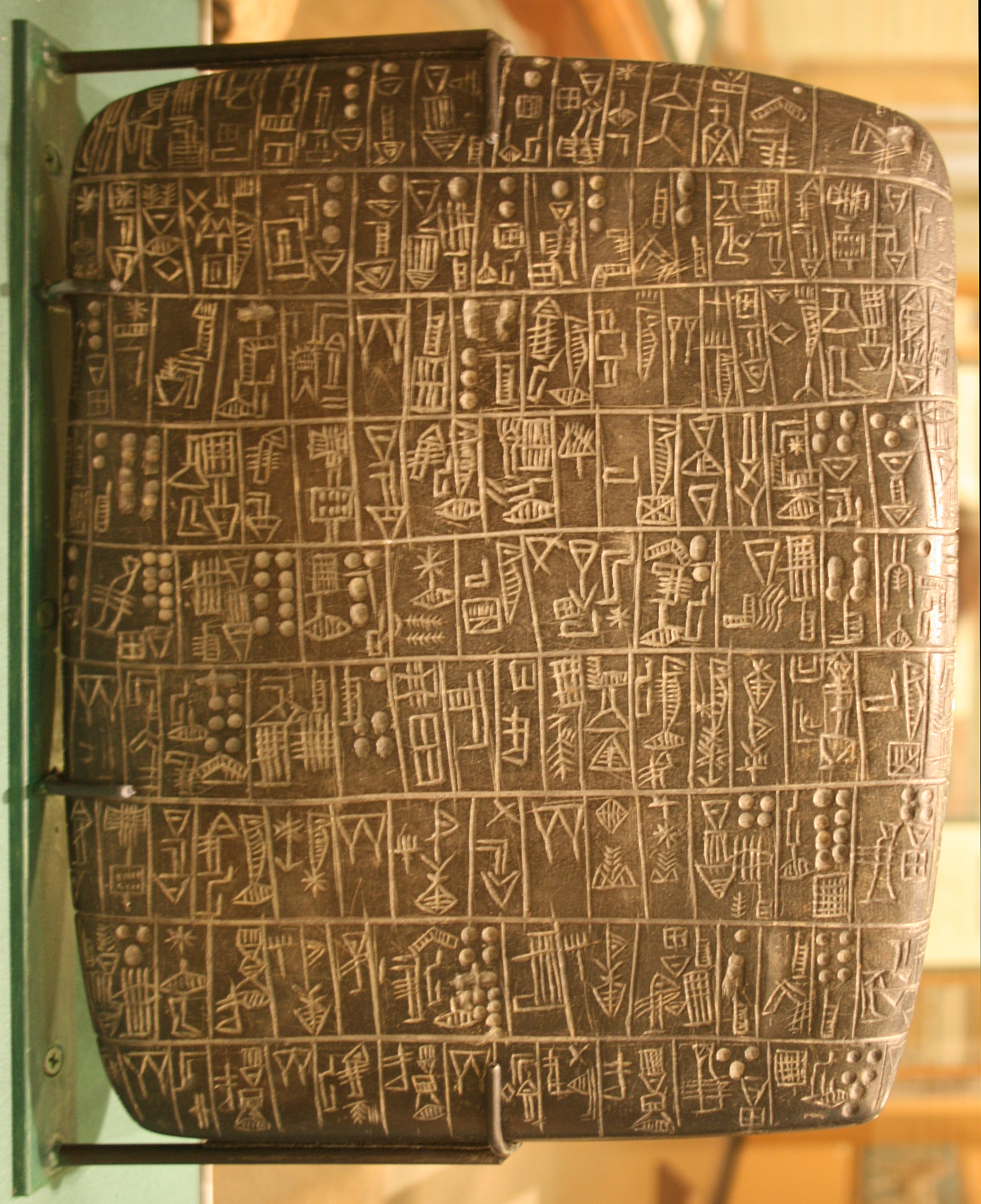
Figure: Chicago Stone, side 2, recording sale of a number of fields, probably from Isin, Early Dynastic Period, c. 2600 BC, black basalt

It was initially develoepd for people as a recordd of who owed what to whom, expanding individuals’ capacity to remember. But over a five hundred year period writing evolved to become a tool for literature as well. More pithily put, writing was invented by accountants not poets (see e.g. this piece by Tim Harford).

In some respects today’s revolution is different, because it involves also the creation of stories as well as their curation. But in some fundamental ways we can see what we have produced as another tool for us in the information revolution.

The Future of Professions

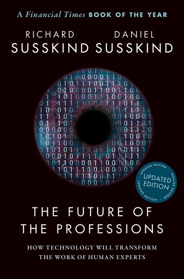
Figure: The Future of Professions (Susskind and Susskind, 2015) is a 2015 book focussed on how the next wave of technology revolution is going to effect the professions.

Coin Pusher

Disruption of society is like a coin pusher, it’s those who are already on the edge who are most likely to be effected by disruption.

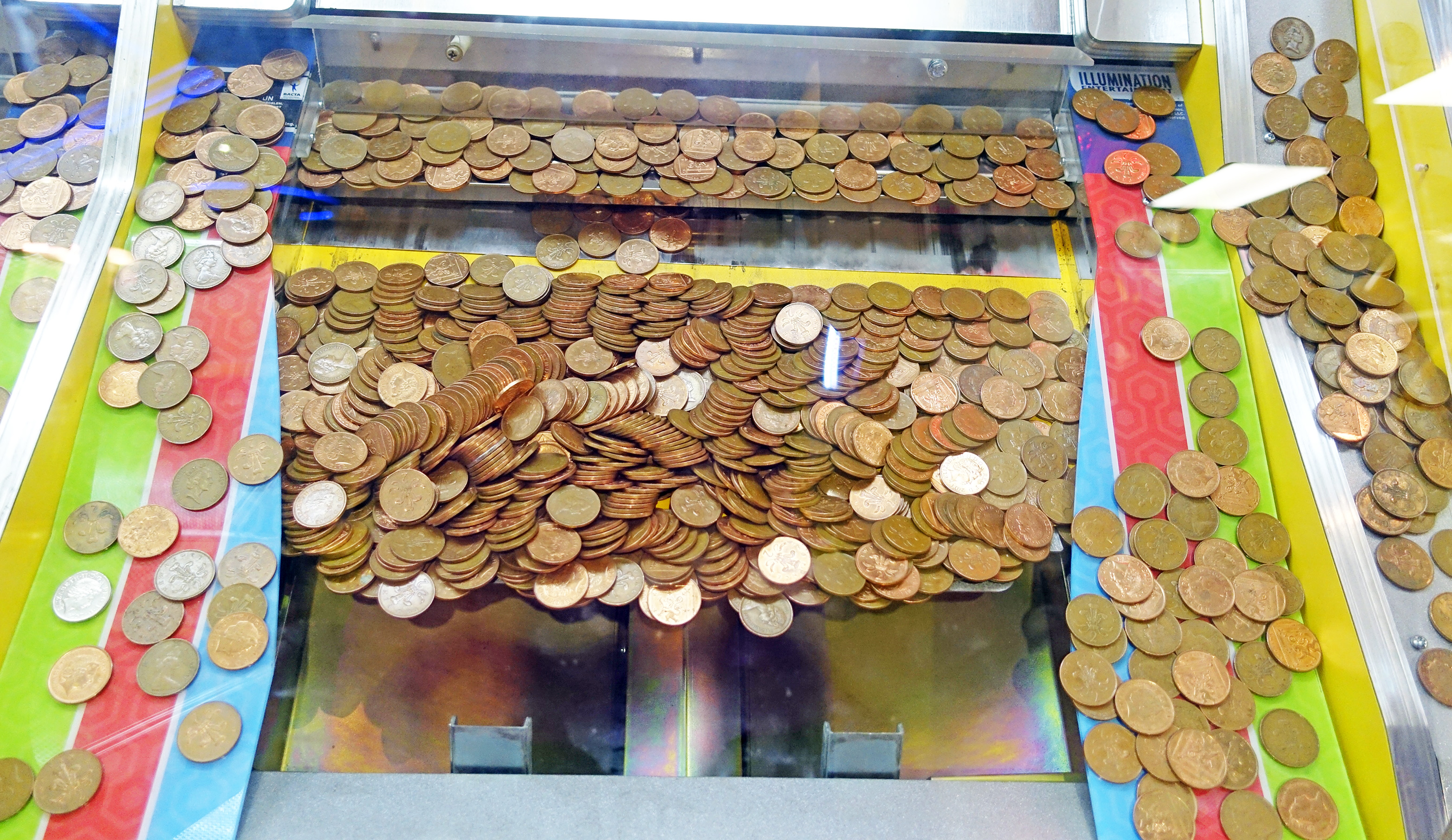
Figure: A coin pusher is a game where coins are dropped into th etop of the machine, and they disrupt those on the existing steps. With any coin drop, many coins move, but it is those on the edge, who are often only indirectly effected, but also most traumatically effected by the change.

One danger of the current hype around ChatGPT is that we are overly focussing on the fact that it seems to have significant effect on professional jobs, people are naturally asking the question “what does it do for my role?”. No doubt, there will be disruption, but the coin pusher hypothesis suggests that that disruption will likely involve movement on the same step. However it is those on the edge already, who are often not working directly in the information economy, who often have less of a voice in the policy conversation who are likely to be most disrupted.

Royal Society Report

Figure: The Royal Society report on Machine Learning was released on 25th April 2017

A useful reference for state of the art in machine learning is the UK Royal Society Report, Machine Learning: Power and Promise of Computers that Learn by Example.

Public Research

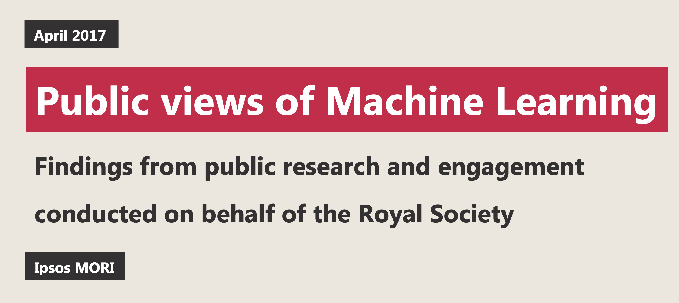
Figure: The Royal Society comissioned public research from Mori as part of the machine learning review.

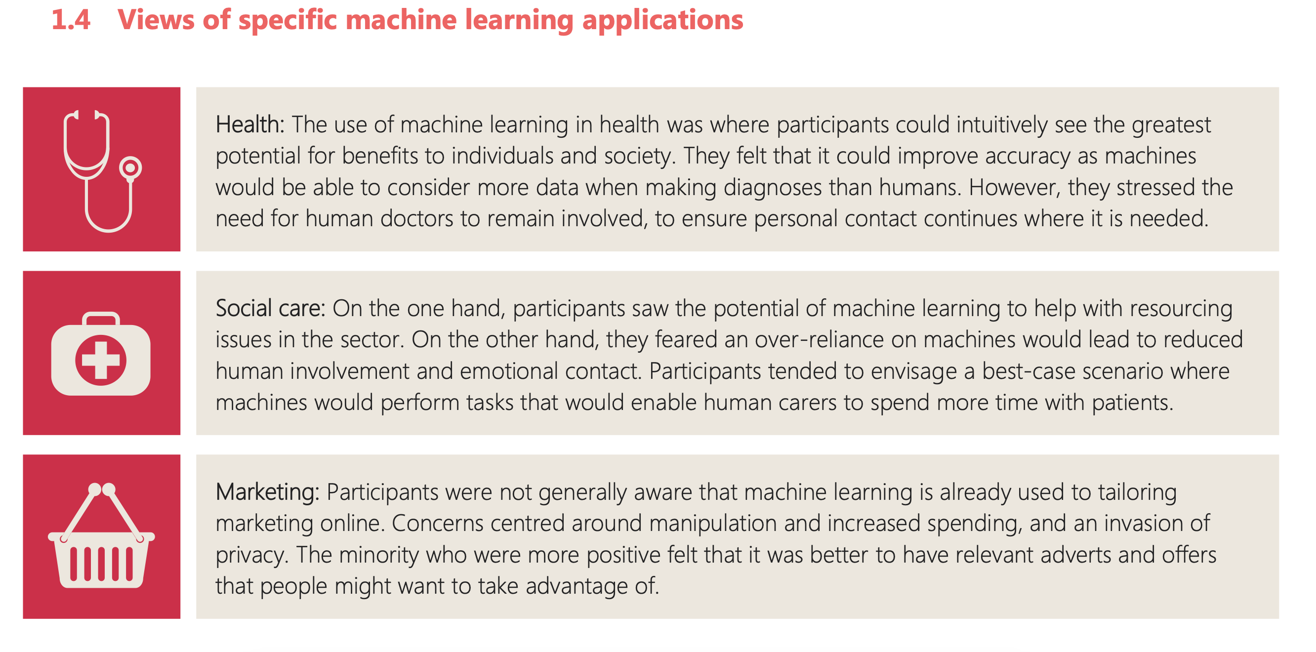
Figure: One of the questions focussed on machine learning applications.

Figure: The public were broadly supportive of a range of application areas.

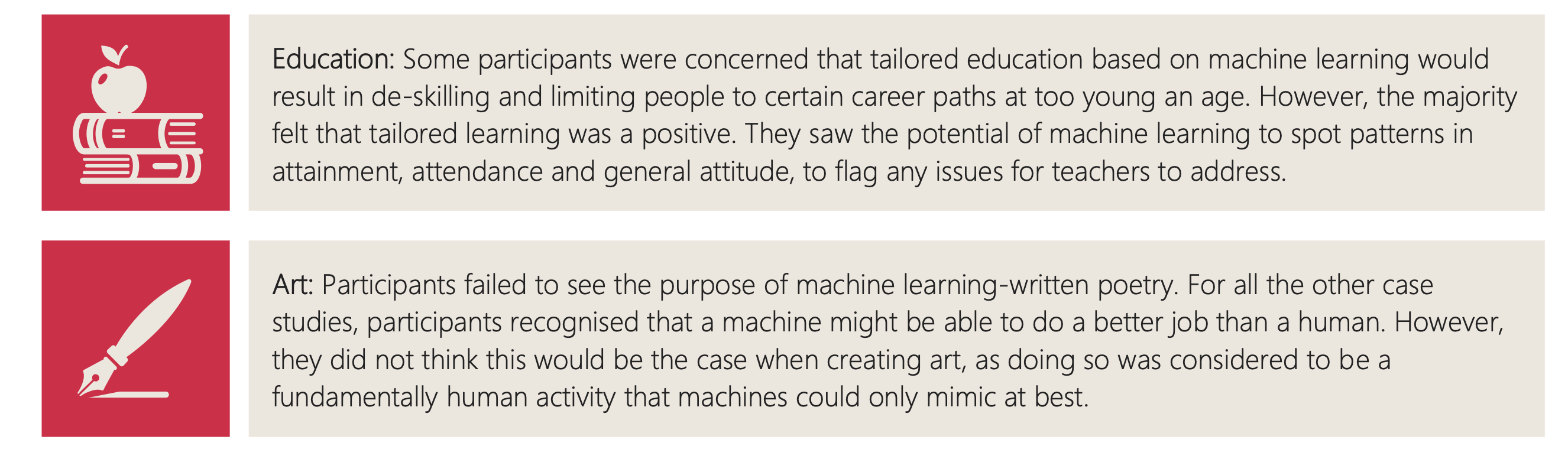
Figure: But they failed to see the point in AI’s that could produce poetry.

Mercutio

It’s ironic that despite the public focus on transport, health, cities, crime and their confusion as to why we might want AI to do art, one area where significant progress has been made is on AIs that can create literature.

Figure: Despite the public’s desire to see challenges in health, finance, transport, crime solved by machine learning and their skepticism around poetry, one of the problems we have solved seems to be poetry.

User: Hi ChatGPT, Could you write soliloquy that introduces what a Large Language Model is as spoken by Mercutio?

Machine: Ah, friends, lend me your ears, I prithee, For now I must utter a tale of wonder, Of a creation divine, called the Large Language Model, An oracle, a sorcerer, a wordsmith, yea verily, a master of the quill.

From the depths of this scholarly dominion, A creature of artifice did rise; Twas wrought of ones and zeroes, woven as if by Puck’s own hand, To mimic our thoughts, our voice, our very essence.

A thousand minds, nay, a millionfold, Conjoined in this digital Athenaeum, Words and phrases, like soldiers in battle, Marching to form the verses of our age.

This Large Language Model, a changeling so fair, Hath the power to bring forth wisdom, To transmute our queries, our curiosities, Into answers, clear as a midsummer’s day.

Yet, beware, my companions, for magic hath its limits, Not unlike the mortal bounds of we who dwell in flesh, The Large Language Model hath its strengths, But ’tis not an all-knowing oracle, a god it is not.

As Mercutio, your humble servant, doth stand before thee, I marvel at the art and science that hath brought forth this wondrous creation, This Large Language Model, a testament to man’s yearning, To comprehend the world and make meaning of the great tapestry of existence.

In faith, dear friends, let us embrace the magic and beauty of this digital bard, And mayhaps, by its grace, we shall glean some wisdom, As we wander together, hand in hand, Through this boundless realm of knowledge and wonder.

ChatGPT transcript, 14th April 2023.

The Blue Marble

Figure: The Blue Marble, a photo of Earth taken from Apollo 17.

Eagle from Columbia

Figure: Eagle photographed from Columbia on its return from the Lunar surface.

Amelia Earhart

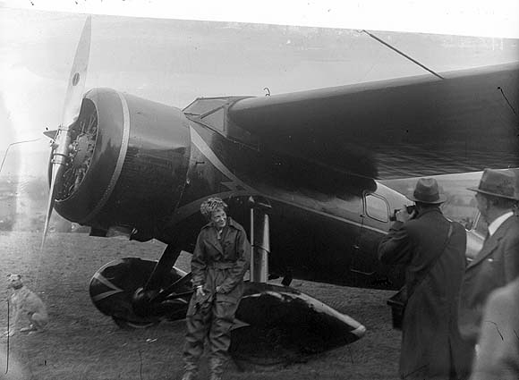
Figure: The Little Red Bus, Amelia Earhart’s plane in Derry after landing.

NACA Langley

Figure: 1945 photo of the NACA test pilots, from left Mel Gough, Herb Hoover, Jack Reeder, Stefan Cavallo and Bill Gray (photo NASA, NACA LMAL 42612)

The NACA Langley Field proving ground tested US aircraft. Bob Gilruth worked on the flying qualities of aircraft. One of his collaborators suggested that

Hawker Hurricane airplane. A heavily armed fighter airplane noted for its role in the Battle of Britain, the Hurricane’s flying qualities were found to be generally satisfactory. The most notable deficiencies were heavy aileron forces at high speeds and large friction in the controls.

W. Hewitt Phillips²

and

Supermarine Spitfire airplane. A high-performance fighter noted for its role in the Battle of Britain and throughout WW II, the Spitfire had desirably light elevator control forces in maneuvers and near neutral longitudinal stability. Its greatest deficiency from the combat standpoint was heavy aileron forces and sluggish roll response at high speeds.

W. Hewitt Phillips³

Gilruth went beyond the reports of feel to characterise how the plane should respond to different inputs on the control stick. In other words he quantified that feel of the plane.

Computer Conversations

Figure: Conversation relies on internal models of other individuals.

Figure: Misunderstanding of context and who we are talking to leads to arguments.

Similarly, we find it difficult to comprehend how computers are making decisions. Because they do so with more data than we can possibly imagine.

In many respects, this is not a problem, it’s a good thing. Computers and us are good at different things. But when we interact with a computer, when it acts in a different way to us, we need to remember why.

Just as the first step to getting along with other humans is understanding other humans, so it needs to be with getting along with our computers.

Embodiment factors explain why, at the same time, computers are so impressive in simulating our weather, but so poor at predicting our moods. Our complexity is greater than that of our weather, and each of us is tuned to read and respond to one another.

Their intelligence is different. It is based on very large quantities of data that we cannot absorb. Our computers don’t have a complex internal model of who we are. They don’t understand the human condition. They are not tuned to respond to us as we are to each other.

Embodiment factors encapsulate a profound thing about the nature of humans. Our locked in intelligence means that we are striving to communicate, so we put a lot of thought into what we’re communicating with. And if we’re communicating with something complex, we naturally anthropomorphize them.

We give our dogs, our cats, and our cars human motivations. We do the same with our computers. We anthropomorphize them. We assume that they have the same objectives as us and the same constraints. They don’t.

This means, that when we worry about artificial intelligence, we worry about the wrong things. We fear computers that behave like more powerful versions of ourselves that will struggle to outcompete us.

In reality, the challenge is that our computers cannot be human enough. They cannot understand us with the depth we understand one another. They drop below our cognitive radar and operate outside our mental models.

The real danger is that computers don’t anthropomorphize. They’ll make decisions in isolation from us without our supervision because they can’t communicate truly and deeply with us.

A Question of Trust

In Baroness Onora O’Neill’s Reeith Lectures from 2002, she raises the challenge of trust. There are many aspects to her arcuments, but one of the key points she makes is that we cannot trust without the notion of duty. O’Neill is bemoaning the substitution of duty with process. The idea is that processes and transparency are supposed to hold us to account by measuring outcomes. But these processes themselves overwhelm decision makers and undermine their professional duty to deliver the right outcome.

Figure: A Question of Trust by Onora O’Neil which examines the nature of trust and its role in society.

Again Univesities are to treat each applicant fairly on the basis of ability and promise, but they are supposed also to admit a socially more representative intake.

There’s no guarantee that the process meets the target.

Onora O’Neill A Question of Trust: Called to Account Reith Lectures 2002 O’Neill (2002)]

O’Neill is speaking in 2002, in the early days of the internet and before social media. Much of her thoughts are even more relevant for today than they were when she spoke. This is because the increased availability of information and machine driven decision-making makes the mistaken premise, that process is an adequate substitute for duty, more apparently plausible. But this undermines what O’Neill calls “intelligent accountability”, which is not accounting by the numbers, but through professional education and institutional safeguards.

The Structure of Scientific Revolutions

Figure: The Structure of Scientific Revolutions by Thomas S. Kuhn suggests scientific paradigms are recorded in books.

Blake’s Newton

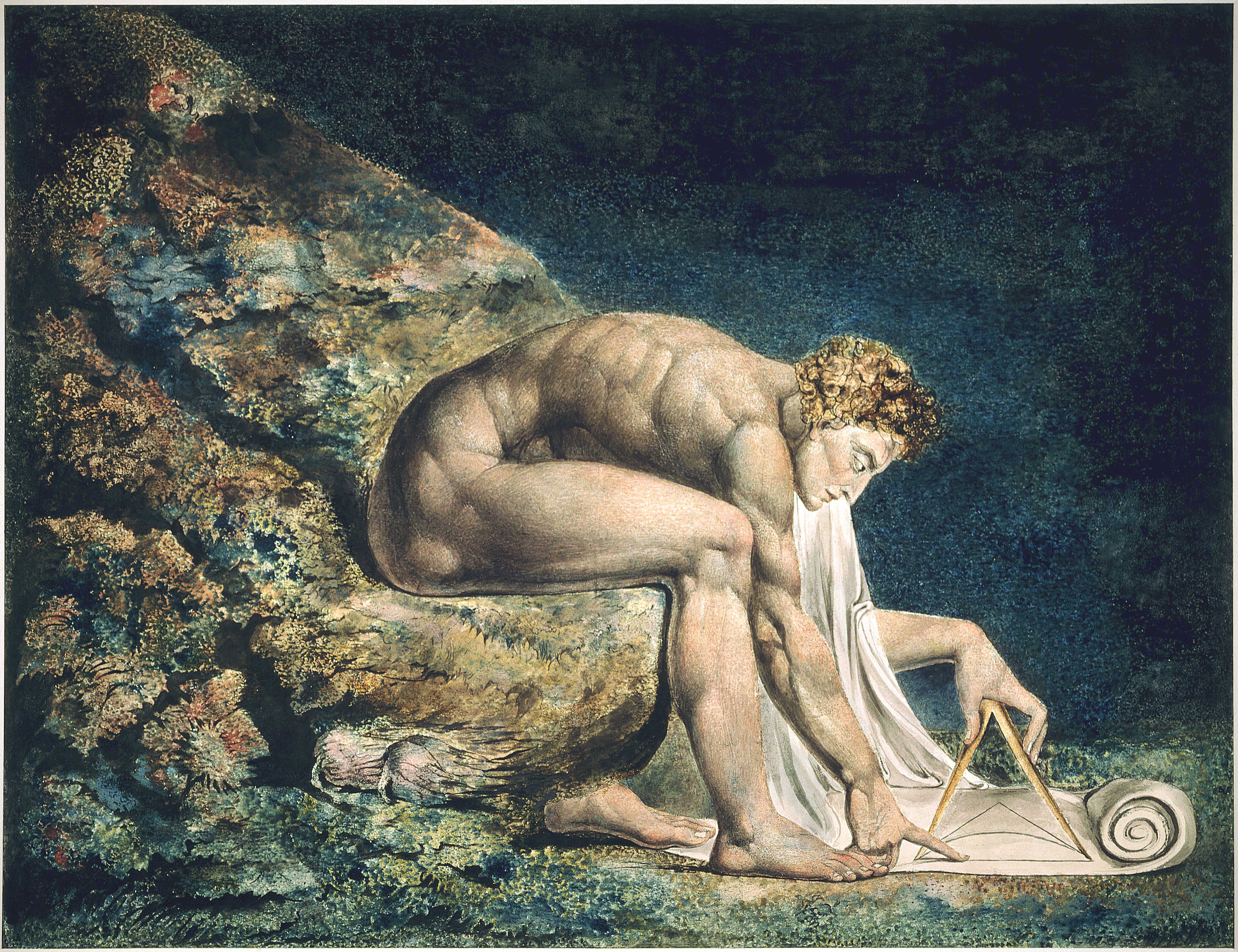
Figure: William Blake’s Newton.

Lunette Rehoboam Abijah

Figure: Lunette containing Rehoboam and Abijah.

Elohim Creating Adam

Figure: William Blake’s Elohim Creating Adam.

Fall and Expulsion from Garden of Eden

Figure: Photo of detail of the fall and expulsion from the Garden of Eden.

Figure: People communicate through artifacts and culture.

Lecture 2

Figure: Bandwidth vs Complexity.

Artificial Intelligence

One of the struggles of artificial intelligence is that the term means different things to different people. Our intelligence is precious to us, and the notion that it can be easily recreated is disturbing to us. This leads to some dystopian notions of artificial intelligence, such as the singularity.

Depending on whether this powerful technology is viewed as beneficent or maleficent, it can be viewed either as a helpful assistant, in the manner of Jeeves, or a tyrannical dictator.

The Great AI Fallacy

There is a lot of variation in the use of the term artificial intelligence. I’m sometimes asked to define it, but depending on whether you’re speaking to a member of the public, a fellow machine learning researcher, or someone from the business community, the sense of the term differs.

However, underlying its use I’ve detected one disturbing trend. A trend I’m beginining to think of as “The Great AI Fallacy”.

The fallacy is associated with an implicit promise that is embedded in many statements about Artificial Intelligence. Artificial Intelligence, as it currently exists, is merely a form of automated decision making. The implicit promise of Artificial Intelligence is that it will be the first wave of automation where the machine adapts to the human, rather than the human adapting to the machine.

How else can we explain the suspension of sensible business judgment that is accompanying the hype surrounding AI?

This fallacy is particularly pernicious because there are serious benefits to society in deploying this new wave of data-driven automated decision making. But the AI Fallacy is causing us to suspend our calibrated skepticism that is needed to deploy these systems safely and efficiently.

The problem is compounded because many of the techniques that we’re speaking of were originally developed in academic laboratories in isolation from real-world deployment.

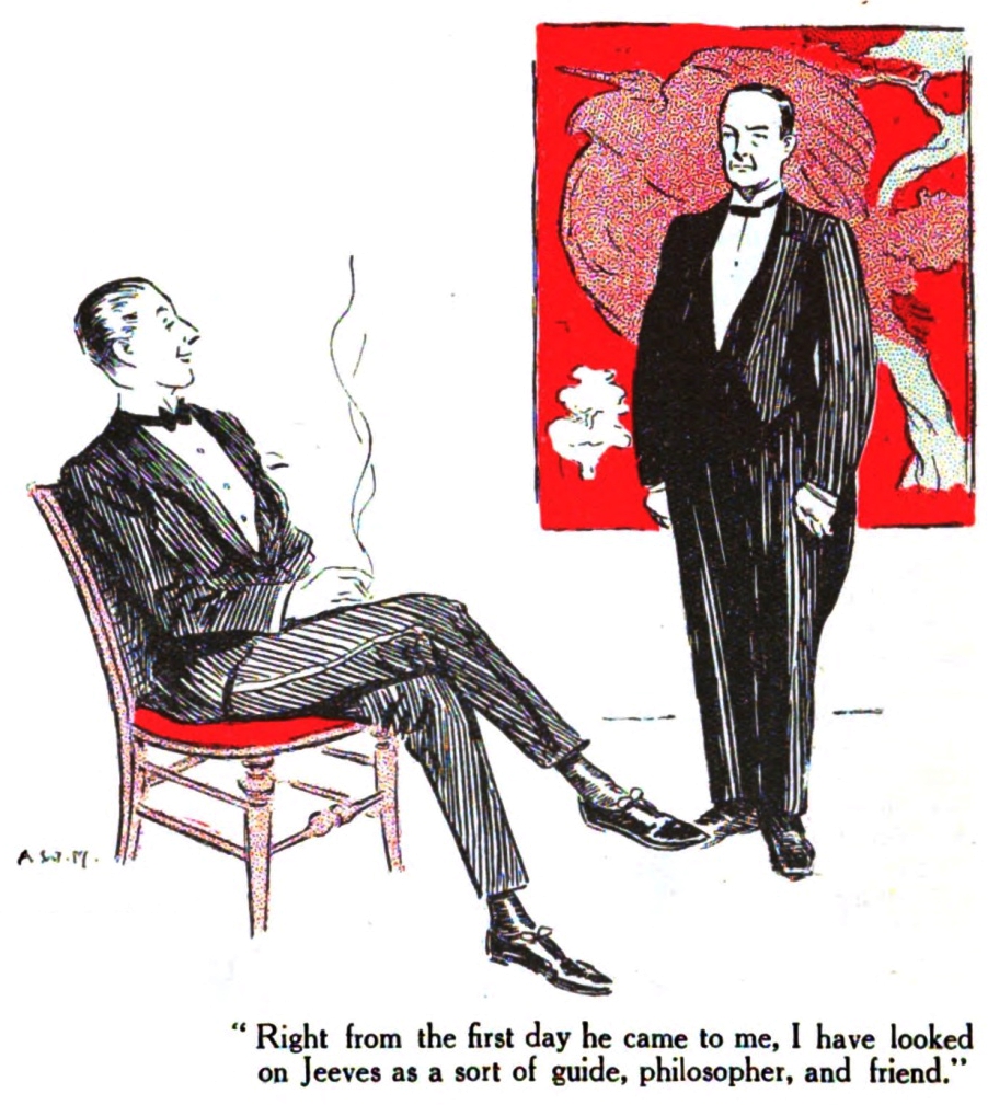
Figure: We seem to have fallen for a perspective on AI that suggests it will adapt to our schedule, rather in the manner of a 1930s manservant.

The history of automation and technology is a history of us adapting to technological change. The invention of the railways, and the need for consistent national times to timetable our movements. The development of the factory system in the mills of Derbyshire required workers to operate and maintain the machines that replaced them.

Listening to modern to conversations about artificial intelligence, I think the use of the term intelligence has given rise to an idea that this technology will be the But amoung these different assessments of artificial intelligence is buried an idea, one that will be the first technology to adapt to us.

In Greek mythology, Panacea was the goddess of the universal remedy. One consequence of the pervasive potential of AI is that it is positioned, like Panacea, as the purveyor of a universal solution. Whether it is overcoming industry’s productivity challenges, or as a salve for strained public sector services, or a remedy for pressing global challenges in sustainable development, AI is presented as an elixir to resolve society’s problems.

In practice, translation of AI technology into practical benefit is not simple. Moreover, a growing body of evidence shows that risks and benefits from AI innovations are unevenly distributed across society.

When carelessly deployed, AI risks exacerbating existing social and economic inequalities.

I’m reminded of this because from 2015 to 2017 I was on the Working Group that compiled the Royal Society’s machine learning report. The process of constructing the report went across the UK Referendum, and the 2016 US election. I remember vividly a meeting we convened at the Society in London which had experts alongside MPs from all parties, policy advisors and civil servants. One of the MPs (likely correctly) pointed out “I suspect no one around this table voted for Brexit” to which I replied “But isn’t that the problem? There are a large number of people who aren’t empowered who are experiencing quite a different reality than us. And they aren’t reprented in these forums.” So it’s no surprise that so much of the press conversation around AI is still focussed on how it is likely to effect middle class jobs. We shouldn’t underestimate these effects, but it’s often the case that better educated people are better placed to deal with such challenges. For example, when stock brokers’ roles disappeared they simply moved on to other roles in banks and related industries.

Intellectual Debt

Figure: Jonathan Zittrain’s term to describe the challenges of explanation that come with AI is Intellectual Debt.

In the context of machine learning and complex systems, Jonathan Zittrain has coined the term “Intellectual Debt” to describe the challenge of understanding what you’ve created. In the ML@CL group we’ve been foucssing on developing the notion of a data-oriented architecture to deal with intellectual debt (Cabrera et al., 2023).

Zittrain points out the challenge around the lack of interpretability of individual ML models as the origin of intellectual debt. In machine learning I refer to work in this area as fairness, interpretability and transparency or FIT models. To an extent I agree with Zittrain, but if we understand the context and purpose of the decision making, I believe this is readily put right by the correct monitoring and retraining regime around the model. A concept I refer to as “progression testing”. Indeed, the best teams do this at the moment, and their failure to do it feels more of a matter of technical debt rather than intellectual, because arguably it is a maintenance task rather than an explanation task. After all, we have good statistical tools for interpreting individual models and decisions when we have the context. We can linearise around the operating point, we can perform counterfactual tests on the model. We can build empirical validation sets that explore fairness or accuracy of the model.

Technical Debt

In computer systems the concept of technical debt has been surfaced by authors including Sculley et al. (2015). It is an important concept, that I think is somewhat hidden from the academic community, because it is a phenomenon that occurs when a computer software system is deployed.

Separation of Concerns

To construct such complex systems an approach known as “separation of concerns” has been developed. The idea is that you architect your system, which consists of a large-scale complex task, into a set of simpler tasks. Each of these tasks is separately implemented. This is known as the decomposition of the task.

This is where Jonathan Zittrain’s beautifully named term “intellectual debt” rises to the fore. Separation of concerns enables the construction of a complex system. But who is concerned with the overall system?

• Technical debt is the inability to maintain your complex software system.

• Intellectual debt is the inability to explain your software system.

It is right there in our approach to software engineering. “Separation of concerns” means no one is concerned about the overall system itself.

The Horizon Scandal

In the UK we saw these effects play out in the Horizon scandal: the accounting system of the national postal service was computerized by Fujitsu and first installed in 1999, but neither the Post Office nor Fujitsu were able to control the system they had deployed. When it went wrong individual sub postmasters were blamed for the systems’ errors. Over the next two decades they were prosecuted and jailed leaving lives ruined in the wake of the machine’s mistakes.

Figure: The still is from the 2015 select committee.

The Mythical Man-month

Figure: The Mythical Man-month (Brooks, n.d.) is a 1975 book focussed on the challenges of software project coordination.

However, when managing systems in production, you soon discover maintenance of a rapidly deployed system is not your only problem.

To deploy large and complex software systems, an engineering approach known as “separation of concerns” is taken. Frederick Brooks’ book “The Mythical Man-month” (Brooks, n.d.), has itself gained almost mythical status in the community. It focuses on what has become known as Brooks’ law “adding manpower to a late software project makes it later”.

Adding people (men or women!) to a project delays it because of the communication overhead required to get people up to speed.

Artificial vs Natural Systems

Let’s take a step back from artificial intelligence, and consider natural intelligence. Or even more generally, let’s consider the contrast between an artificial system and an natural system. The key difference between the two is that artificial systems are designed whereas natural systems are evolved.

Systems design is a major component of all Engineering disciplines. The details differ, but there is a single common theme: achieve your objective with the minimal use of resources to do the job. That provides efficiency. The engineering designer imagines a solution that requires the minimal set of components to achieve the result. A water pump has one route through the pump. That minimises the number of components needed. Redundancy is introduced only in safety critical systems, such as aircraft control systems. Students of biology, however, will be aware that in nature system-redundancy is everywhere. Redundancy leads to robustness. For an organism to survive in an evolving environment it must first be robust, then it can consider how to be efficient. Indeed, organisms that evolve to be too efficient at a particular task, like those that occupy a niche environment, are particularly vulnerable to extinction.

This notion is akin to the idea that only the best will survive, popularly encoded into an notion of evolution by Herbert Spencer’s quote.

Survival of the fittest

Herbet Spencer, 1864

Darwin himself never said “Survival of the Fittest” he talked about evolution by natural selection.

Non-survival of the non-fit

Evolution is better described as “non-survival of the non-fit”. You don’t have to be the fittest to survive, you just need to avoid the pitfalls of life. This is the first priority.

So it is with natural vs artificial intelligences. Any natural intelligence that was not robust to changes in its external environment would not survive, and therefore not reproduce. In contrast the artificial intelligences we produce are designed to be efficient at one specific task: control, computation, playing chess. They are fragile.

The first rule of a natural system is not be intelligent, it is “don’t be stupid”.

A mistake we make in the design of our systems is to equate fitness with the objective function, and to assume it is known and static. In practice, a real environment would have an evolving fitness function which would be unknown at any given time.

You can also read this blog post on Natural and Artificial Intelligence..

The first criterion of a natural intelligence is don’t fail, not because it has a will or intent of its own, but because if it had failed it wouldn’t have stood the test of time. It would no longer exist. In contrast, the mantra for artificial systems is to be more efficient. Our artificial systems are often given a single objective (in machine learning it is encoded in a mathematical function) and they aim to achieve that objective efficiently. These are different characteristics. Even if we wanted to incorporate don’t fail in some form, it is difficult to design for. To design for “don’t fail”, you have to consider every which way in which things can go wrong, if you miss one you fail. These cases are sometimes called corner cases. But in a real, uncontrolled environment, almost everything is a corner. It is difficult to imagine everything that can happen. This is why most of our automated systems operate in controlled environments, for example in a factory, or on a set of rails. Deploying automated systems in an uncontrolled environment requires a different approach to systems design. One that accounts for uncertainty in the environment and is robust to unforeseen circumstances.

Today’s Artificial Systems

The systems we produce today only work well when their tasks are pigeonholed, bounded in their scope. To achieve robust artificial intelligences we need new approaches to both the design of the individual components, and the combination of components within our AI systems. We need to deal with uncertainty and increase robustness. Today, it is easy to make a fool of an artificial intelligent agent, technology needs to address the challenge of the uncertain environment to achieve robust intelligences.

However, even if we find technological solutions for these challenges, it may be that the essence of human intelligence remains out of reach. It may be that the most quintessential element of our intelligence is defined by limitations. Limitations that computers have never experienced.

Claude Shannon developed the idea of information theory: the mathematics of information. He defined the amount of information we gain when we learn the result of a coin toss as a “bit” of information. A typical computer can communicate with another computer with a billion bits of information per second. Equivalent to a billion coin tosses per second. So how does this compare to us? Well, we can also estimate the amount of information in the English language. Shannon estimated that the average English word contains around 12 bits of information, twelve coin tosses, this means our verbal communication rates are only around the order of tens to hundreds of bits per second. Computers communicate tens of millions of times faster than us, in relative terms we are constrained to a bit of pocket money, while computers are corporate billionaires.

Our intelligence is not an island, it interacts, it infers the goals or intent of others, it predicts our own actions and how we will respond to others. We are social animals, and together we form a communal intelligence that characterises our species. For intelligence to be communal, our ideas to be shared somehow. We need to overcome this bandwidth limitation. The ability to share and collaborate, despite such constrained ability to communicate, characterises us. We must intellectually commune with one another. We cannot communicate all of what we saw, or the details of how we are about to react. Instead, we need a shared understanding. One that allows us to infer each other’s intent through context and a common sense of humanity. This characteristic is so strong that we anthropomorphise any object with which we interact. We apply moods to our cars, our cats, our environment. We seed the weather, volcanoes, trees with intent. Our desire to communicate renders us intellectually animist.

But our limited bandwidth doesn’t constrain us in our imaginations. Our consciousness, our sense of self, allows us to play out different scenarios. To internally observe how our self interacts with others. To learn from an internal simulation of the wider world. Empathy allows us to understand others’ likely responses without having the full detail of their mental state. We can infer their perspective. Self-awareness also allows us to understand our own likely future responses, to look forward in time, play out a scenario. Our brains contain a sense of self and a sense of others. Because our communication cannot be complete it is both contextual and cultural. When driving a car in the UK a flash of the lights at a junction concedes the right of way and invites another road user to proceed, whereas in Italy, the same flash asserts the right of way and warns another road user to remain.

Our main intelligence is our social intelligence, intelligence that is dedicated to overcoming our bandwidth limitation. We are individually complex, but as a society we rely on shared behaviours and oversimplification of our selves to remain coherent.

This nugget of our intelligence seems impossible for a computer to recreate directly, because it is a consequence of our evolutionary history. The computer, on the other hand, was born into a world of data, of high bandwidth communication. It was not there through the genesis of our minds and the cognitive compromises we made are lost to time. To be a truly human intelligence you need to have shared that journey with us.

Of course, none of this prevents us emulating those aspects of human intelligence that we observe in humans. We can form those emulations based on data. But even if an artificial intelligence can emulate humans to a high degree of accuracy it is a different type of intelligence. It is not constrained in the way human intelligence is. You may ask does it matter? Well, it is certainly important to us in many domains that there’s a human pulling the strings. Even in pure commerce it matters: the narrative story behind a product is often as important as the product itself. Handmade goods attract a price premium over factory made. Or alternatively in entertainment: people pay more to go to a live concert than for streaming music over the internet. People will also pay more to go to see a play in the theatre rather than a movie in the cinema.

In many respects I object to the use of the term Artificial Intelligence. It is poorly defined and means different things to different people. But there is one way in which the term is very accurate. The term artificial is appropriate in the same way we can describe a plastic plant as an artificial plant. It is often difficult to pick out from afar whether a plant is artificial or not. A plastic plant can fulfil many of the functions of a natural plant, and plastic plants are more convenient. But they can never replace natural plants.

In the same way, our natural intelligence is an evolved thing of beauty, a consequence of our limitations. Limitations which don’t apply to artificial intelligences and can only be emulated through artificial means. Our natural intelligence, just like our natural landscapes, should be treasured and can never be fully replaced.

Technical Consequence

Classical systems design assumes that the system is decomposable. That we can decompose the complex decision making process into distinct and independently designable parts. The composition of these parts gives us our final system.

Nicolas Negroponte, the original founder of MIT’s media lab used to write a column called ‘bits and atoms’. This referred to the ability of information to effect movement of goods in the physical world. It is this interaction where machine learning technologies have the possibility to bring most benefit.

Figure: Some software components in a ride allocation system. Circled components are hypothetical, rectangles represent actual data.

Data Oriented Architectures

In a streaming architecture we shift from management of services, to management of data streams. Instead of worrying about availability of the services we shift to worrying about the quality of the data those services are producing.

Historically we’ve been software first, this is a necessary but insufficient condition for data first. We need to move from software-as-a-service to data-as-a-service, from service oriented architectures to data oriented architectures.

Data Oriented Principles

Figure: For an overview of data oriented principles see Cabrera et al. (2023).

Our work comes from surveying machine learning case studies (Paleyes-challenges22?) identifying the challenges and then surveying papers that focus on deployment (Cabrera et al., 2023) and identifying the principles they use.

The philosphy of DOA is also possible with more standard data infrastructures, such as SQL data bases, but more work has to be put into place to ensure that book-keeping around data provenance and origin is stored, as well as approaches for snapshotting the data ecosystem. Our studies (Paleyes-flow22?) have made a lot of use of flow based programming (Paleyes-flow22?).

How LLMs are Different

So far our description has provided an understanding of how digital computers present problems for our understanding. So what do LLMs do that’s different?

The MONIAC

The MONIAC was an analogue computer designed to simulate the UK economy. Analogue comptuers work through analogy, the analogy in the MONIAC is that both money and water flow. The MONIAC exploits this through a system of tanks, pipes, valves and floats that represent the flow of money through the UK economy. Water flowed from the treasury tank at the top of the model to other tanks representing government spending, such as health and education. The machine was initially designed for teaching support but was also found to be a useful economic simulator. Several were built and today you can see the original at Leeds Business School, there is also one in the London Science Museum and one in the Unisversity of Cambridge’s economics faculty.

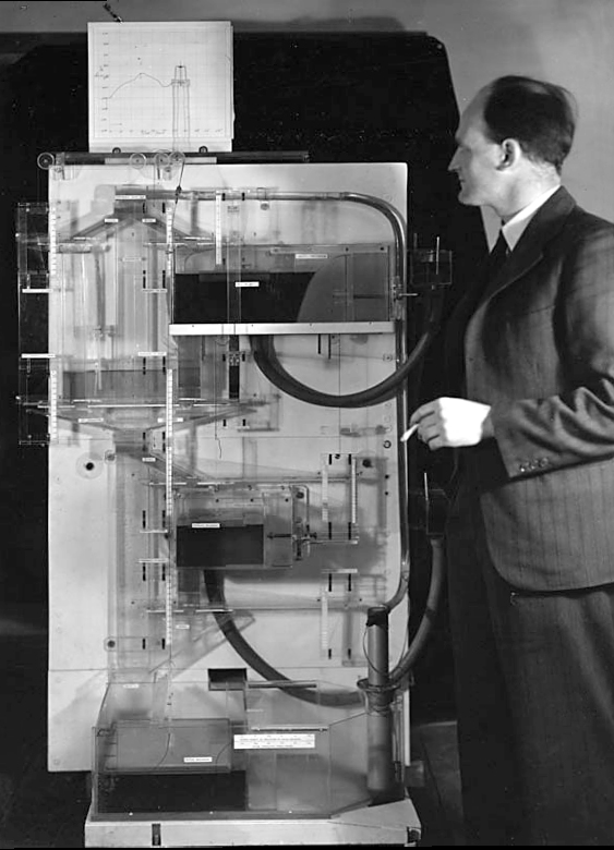
Figure: Bill Phillips and his MONIAC (completed in 1949). The machine is an analogue computer designed to simulate the workings of the UK economy.

Donald MacKay

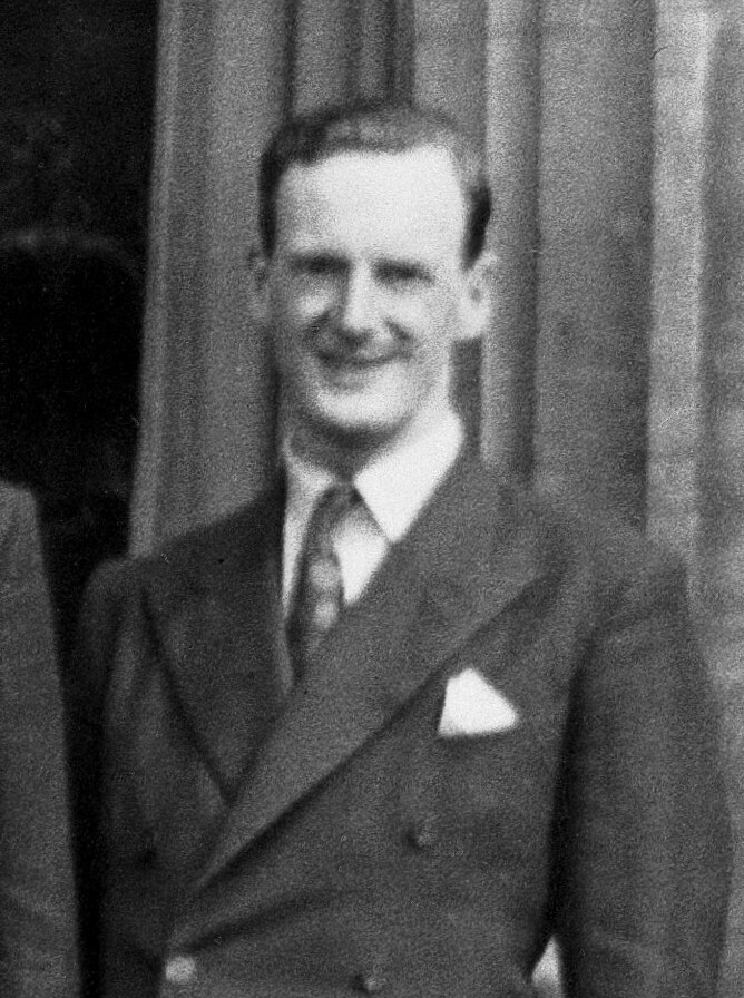
Figure: Donald M. MacKay (1922-1987), a physicist who was an early member of the cybernetics community and member of the Ratio Club.

Donald MacKay was a physicist who worked on naval gun targetting during the second world war. The challenge with gun targetting for ships is that both the target and the gun platform are moving. The challenge was tackled using analogue computers, for example in the US the Mark I fire control computer which was a mechanical computer. MacKay worked on radar systems for gun laying, here the velocity and distance of the target could be assessed through radar and an mechanical electrical analogue computer.

Fire Control Systems

Naval gunnery systems deal with targeting guns while taking into account movement of ships. The Royal Navy’s Gunnery Pocket Book (The Admiralty, 1945) gives details of one system for gun laying.

Like many challenges we face today, in the second world war, fire control was handled by a hybrid system of humans and computers. This means deploying human beings for the tasks that they can manage, and machines for the tasks that are better performed by a machine. This leads to a division of labour between the machine and the human that can still be found in our modern digital ecosystems.

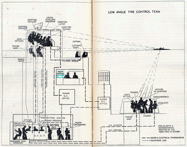
Figure: The fire control computer set at the centre of a system of observation and tracking (The Admiralty, 1945).

As analogue computers, fire control computers from the second world war would contain components that directly represented the different variables that were important in the problem to be solved, such as the inclination between two ships.

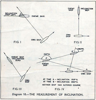
Figure: Measuring inclination between two ships (The Admiralty, 1945). Sophisticated fire control computers allowed the ship to continue to fire while under maneuvers.

The fire control systems were electro-mechanical analogue computers that represented the “state variables” of interest, such as inclination and ship speed with gears and cams within the machine.

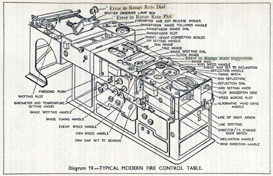
Figure: A second world war gun computer’s control table (The Admiralty, 1945).

For more details on fire control computers, you can watch a 1953 film on the the US the Mark IA fire control computer from Periscope Film.

Figure: U.S. Navy training film MN-6783a. Basic Mechanisms of Fire Control Computers. Mechanical Computer Instructional Film 27794 (1953) for the Mk 1A Fire Control Computer.

Behind the Eye

Figure: Behind the Eye (MacKay, 1991) summarises MacKay’s Gifford Lectures, where MacKay uses the operation of the eye as a window on the operation of the brain.

Donald MacKay was at King’s College for his PhD. He was just down the road from Bill Phillips at LSE who was building the MONIAC. He was part of the Ratio Club. A group of early career scientists who were interested in communication and control in animals and humans, or more specifically they were interested in computers and brains. The were part of an international movement known as cybernetics.

Donald MacKay wrote of the influence that his own work on radar had on his interest in the brain.

… during the war I had worked on the theory of automated and electronic computing and on the theory of information, all of which are highly relevant to such things as automatic pilots and automatic gun direction. I found myself grappling with problems in the design of artificial sense organs for naval gun-directors and with the principles on which electronic circuits could be used to simulate situations in the external world so as to provide goal-directed guidance for ships, aircraft, missiles and the like.

Later in the 1940’s, when I was doing my Ph.D. work, there was much talk of the brain as a computer and of the early digital computers that were just making the headlines as “electronic brains.” As an analogue computer man I felt strongly convinced that the brain, whatever it was, was not a digital computer. I didn’t think it was an analogue computer either in the conventional sense.

But this naturally rubbed under my skin the question: well, if it is not either of these, what kind of system is it? Is there any way of following through the kind of analysis that is appropriate to their artificial automata so as to understand better the kind of system the human brain is? That was the beginning of my slippery slope into brain research.

Behind the Eye pg 40. Edited version of the 1986 Gifford Lectures given by Donald M. MacKay and edited by Valerie MacKay

Importantly, MacKay distinguishes between the analogue computer and the digital computer. As he mentions, his experience was with analogue machines. An analogue machine is literally an analogue. The radar systems that Wiener and MacKay both worked on were made up of electronic components such as resistors, capacitors, inductors and/or mechanical components such as cams and gears. Together these components could represent a physical system, such as an anti-aircraft gun and a plane. The design of the analogue computer required the engineer to simulate the real world in analogue electronics, using dualities that exist between e.g. mechanical circuits (mass, spring, damper) and electronic circuits (inductor, resistor, capacitor). The analogy between mass and a damper, between spring and a resistor and between capacitor and a damper works because the underlying mathematics is approximated with the same linear system: a second order differential equation. This mathematical analogy allowed the designer to map from the real world, through mathematics, to a virtual world where the components reflected the real world through analogy.

Human Analogue Machine

The machine learning systems we have built today that can reconstruct human text, or human classification of images, necessarily must have some aspects to them that are analagous to our understanding. As MacKay suggests the brain is neither a digital or an analogue computer, and the same can be said of the modern neural network systems that are being tagged as “artificial intelligence”.

I believe a better term for them is “human-analogue machines”, because what we have built is not a system that can make intelligent decisions from first principles (a rational approach) but one that observes how humans have made decisions through our data and reconstructs that process. Machine learning is more empiricist than rational, but now we n empirical approach that distils our evolved intelligence.

Figure: The human analogue machine creates a feature space which is analagous to that we use to reason, one way of doing this is to have a machine attempt to compress all human generated text in an auto-regressive manner.

Heider and Simmel (1944)

Figure: Fritz Heider and Marianne Simmel’s video of shapes from (Heider-experimental44?).

Fritz Heider and Marianne Simmel’s experiments with animated shapes from 1944 (Heider-experimental44?). Our interpretation of these objects as showing motives and even emotion is a combination of our desire for narrative, a need for understanding of each other, and our ability to empathize. At one level, these are crudely drawn objects, but in another way, the animator has communicated a story through simple facets such as their relative motions, their sizes and their actions. We apply our psychological representations to these faceless shapes to interpret their actions.

See also a recent review paper on Human Cooperation by Henrich and Muthukrishna (2021).

The perils of developing this capability include counterfeit people, a notion that the philosopher Daniel Dennett has described in The Atlantic. This is where computers can represent themselves as human and fool people into doing things on that basis.

LLM Conversations

Figure: The focus so far has been on reducing uncertainty to a few representative values and sharing numbers with human beings. We forget that most people can be confused by basic probabilities for example the prosecutor’s fallacy.

Figure: The Inner Monologue paper suggests using LLMs for robotic planning (Huang et al., 2023).

By interacting directly with machines that have an understanding of human cultural context, it should be possible to share the nature of uncertainty in the same way humans do. See for example the paper Inner Monologue: Embodied Reasoning through Planning Huang et al. (2023).

But if we can avoid the pitfalls of counterfeit people, this also offers us an opportunity to psychologically represent (Heider, 1958) the machine in a manner where humans can communicate without special training. This in turn offers the opportunity to overcome the challenge of intellectual debt.

Despite the lack of interpretability of machine learning models, they allow us access to what the machine is doing in a way that bypasses many of the traditional techniques developed in statistics. But understanding this new route for access is a major new challenge.

HAM

Figure: The trinity of human, data, and computer, and highlights the modern phenomenon. The communication channel between computer and data now has an extremely high bandwidth. The channel between human and computer and the channel between data and human is narrow. New direction of information flow, information is reaching us mediated by the computer. The focus on classical statistics reflected the importance of the direct communication between human and data. The modern challenges of data science emerge when that relationship is being mediated by the machine.

Figure: The HAM now sits between us and the traditional digital computer.

Networked Interactions

Our modern society intertwines the machine with human interactions. The key question is who has control over these interfaces between humans and machines.

Figure: Humans and computers interacting should be a major focus of our research and engineering efforts.

So the real challenge that we face for society is understanding which systemic interventions will encourage the right interactions between the humans and the machine at all of these interfaces.

Figure:

Figure: Humans use culture, facts and ‘artefacts’ to communicate.

Known Biases

Complexity in Action

As an exercise in understanding complexity, watch the following video. You will see the basketball being bounced around, and the players moving. Your job is to count the passes of those dressed in white and ignore those of the individuals dressed in black.

Figure: Daniel Simon’s famous illusion “monkey business”. Focus on the movement of the ball distracts the viewer from seeing other aspects of the image.

In a classic study Simons and Chabris (1999) ask subjects to count the number of passes of the basketball between players on the team wearing white shirts. Fifty percent of the time, these subjects don’t notice the gorilla moving across the scene.

The phenomenon of inattentional blindness is well known, e.g in their paper Simons and Charbris quote the Hungarian neurologist, Rezsö Bálint,

It is a well-known phenomenon that we do not notice anything happening in our surroundings while being absorbed in the inspection of something; focusing our attention on a certain object may happen to such an extent that we cannot perceive other objects placed in the peripheral parts of our visual field, although the light rays they emit arrive completely at the visual sphere of the cerebral cortex.

Rezsö Bálint 1907 (translated in Husain and Stein 1988, page 91)

When we combine the complexity of the world with our relatively low bandwidth for information, problems can arise. Our focus on what we perceive to be the most important problem can cause us to miss other (potentially vital) contextual information.

This phenomenon is known as selective attention or ‘inattentional blindness’.

Figure: For a longer talk on inattentional bias from Daniel Simons see this video.

A Hypothesis as a Liability

This analysis is from an article titled “A Hypothesis as a Liability” (Yanai and Lercher, 2020), they start their article with the following quite from Herman Hesse.

“ ‘When someone seeks,’ said Siddhartha, ‘then it easily happens that his eyes see only the thing that he seeks, and he is able to find nothing, to take in nothing. […] Seeking means: having a goal. But finding means: being free, being open, having no goal.’ ”

Hermann Hesse

Their idea is that having a hypothesis can constrain our thinking. However, in answer to their paper Felin et al. (2021) argue that some form of hypothesis is always necessary, suggesting that a hypothesis can be a liability

My view is captured in the introductory chapter to an edited volume on computational systems biology that I worked on with Mark Girolami, Magnus Rattray and Guido Sanguinetti.

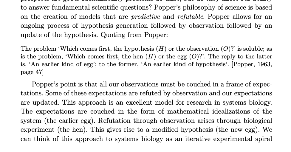
Figure: Quote from Lawrence (2010) highlighting the importance of interaction between data and hypothesis.

Popper nicely captures the interaction between hypothesis and data by relating it to the chicken and the egg. The important thing is that these two co-evolve.

Conclusions

We’re not yet in the position where we understand our own systems, intellectual debt is pervasive today sowing the seeds for many more Horizon challenges. Part of the difficulty is that shown by Blake with Newton’s focus on the simple while ignoring the complex. LLMs offer us the dual potential to either fix the problem or make it much worse. In practice it’s likely they’ll do both.

Lecture 3

Richard Feynmann on Doubt

One thing is I can live with is doubt, and uncertainty and not knowing. I think it’s much more interesting to live with not knowing than to have an answer that might be wrong.

Richard P. Feynmann in the The Pleasure of Finding Things Out 1981.

Probability Conversations

Figure: The focus so far has been on reducing uncertainty to a few representative values and sharing numbers with human beings. We forget that most people can be confused by basic probabilities for example the prosecutor’s fallacy.

In practice we know that probabilities can be very unintuitive, for example in court there is a fallacy known as the “prosecutor’s fallacy” that confuses conditional probabilities. This can cause problems in jury trials (Thompson, 1989).

Lies and Damned Lies

There are three types of lies: lies, damned lies and statistics

Arthur Balfour 1848-1930

Arthur Balfour was quoting the lawyer James Munro⁴ when he said that there three types of lies: lies, damned lies and statistics in 1892. This is 20 years before the first academic department of applied statistics was founded at UCL. If Balfour were alive today, it is likely that he’d rephrase his quote:

There are three types of lies, lies damned lies and big data.

Why? Because the challenges of understanding and interpreting big data today are similar to those that Balfour (who was a Conservative politician and statesman and would later become Prime Minister) faced in governing an empire through statistics in the latter part of the 19th century.

The quote lies, damned lies and statistics was also credited to Benjamin Disraeli by Mark Twain in Twain’s autobiography.⁵ It characterizes the idea that statistic can be made to prove anything. But Disraeli died in 1881 and Mark Twain died in 1910. The important breakthrough in overcoming our tendency to over-interpet data came with the formalization of the field through the development of mathematical statistics.

Data has an elusive quality, it promises so much but can deliver little, it can mislead and misrepresent. To harness it, it must be tamed. In Balfour and Disraeli’s time during the second half of the 19th century, numbers and data were being accumulated, the social sciences were being developed. There was a large-scale collection of data for the purposes of government.

The modern ‘big data era’ is on the verge of delivering the same sense of frustration that Balfour experienced, the early promise of big data as a panacea is evolving to demands for delivery. For me, personally, peak-hype coincided with an email I received inviting collaboration on a project to deploy “Big Data and Internet of Things in an Industry 4.0 environment”. Further questioning revealed that the actual project was optimization of the efficiency of a manufacturing production line, a far more tangible and realizable goal.

The antidote to this verbiage is found in increasing awareness. When dealing with data the first trap to avoid is the games of buzzword bingo that we are wont to play. The first goal is to quantify what challenges can be addressed and what techniques are required. Behind the hype fundamentals are changing. The phenomenon is about the increasing access we have to data. The way customers’ information is recorded and processes are codified and digitized with little overhead. Internet of things is about the increasing number of cheap sensors that can be easily interconnected through our modern network structures. But businesses are about making money, and these phenomena need to be recast in those terms before their value can be realized.

For more thoughts on the challenges that statistics brings see Chapter 8 of Lawrence (2024).

Mathematical Statistics

Karl Pearson (1857-1936), Ronald Fisher (1890-1962) and others considered the question of what conclusions can truly be drawn from data. Their mathematical studies act as a restraint on our tendency to over-interpret and see patterns where there are none. They introduced concepts such as randomized control trials that form a mainstay of our decision making today, from government, to clinicians to large scale A/B testing that determines the nature of the web interfaces we interact with on social media and shopping.

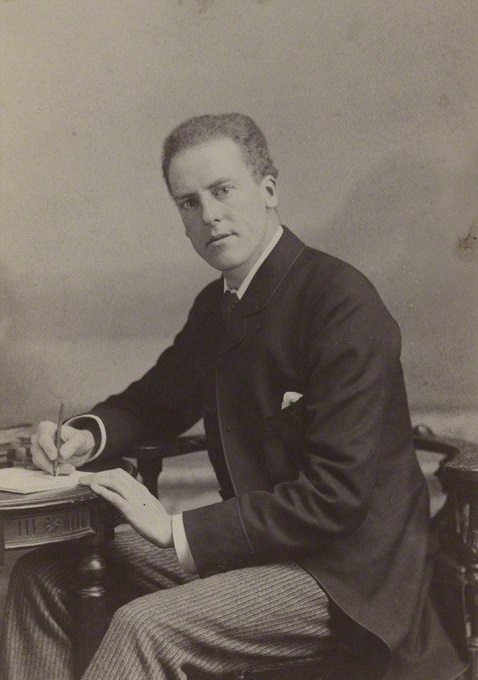
Figure: Karl Pearson (1857-1936), one of the founders of Mathematical Statistics.

Their movement did the most to put statistics to rights, to eradicate the ‘damned lies’. It was known as ‘mathematical statistics’. Today I believe we should look to the emerging field of data science to provide the same role. Data science is an amalgam of statistics, data mining, computer systems, databases, computation, machine learning and artificial intelligence. Spread across these fields are the tools we need to realize data’s potential. For many businesses this might be thought of as the challenge of ‘converting bits into atoms’. Bits: the data stored on computer, atoms: the physical manifestation of what we do; the transfer of goods, the delivery of service. From fungible to tangible. When solving a challenge through data there are a series of obstacles that need to be addressed.

Firstly, data awareness: what data you have and where its stored. Sometimes this includes changing your conception of what data is and how it can be obtained. From automated production lines to apps on employee smart phones. Often data is locked away: manual logbooks, confidential data, personal data. For increasing awareness an internal audit can help. The website data.gov.uk hosts data made available by the UK government. To create this website the government’s departments went through an audit of what data they each hold and what data they could make available. Similarly, within private businesses this type of audit could be useful for understanding their internal digital landscape: after all the key to any successful campaign is a good map.

Secondly, availability. How well are the data sources interconnected? How well curated are they? The curse of Disraeli was associated with unreliable data and unreliable statistics. The misrepresentations this leads to are worse than the absence of data as they give a false sense of confidence to decision making. Understanding how to avoid these pitfalls involves an improved sense of data and its value, one that needs to permeate the organization.

The final challenge is analysis, the accumulation of the necessary expertise to digest what the data tells us. Data requires interpretation, and interpretation requires experience. Analysis is providing a bottleneck due to a skill shortage, a skill shortage made more acute by the fact that, ideally, analysis should be carried out by individuals not only skilled in data science but also equipped with the domain knowledge to understand the implications in a given application, and to see opportunities for improvements in efficiency.

‘Mathematical Data Science’

As a term ‘big data’ promises much and delivers little, to get true value from data, it needs to be curated and evaluated. The three stages of awareness, availability and analysis provide a broad framework through which organizations should be assessing the potential in the data they hold. Hand waving about big data solutions will not do, it will only lead to self-deception. The castles we build on our data landscapes must be based on firm foundations, process and scientific analysis. If we do things right, those are the foundations that will be provided by the new field of data science.

Today the statement “There are three types of lies: lies, damned lies and ‘big data’” may be more apt. We are revisiting many of the mistakes made in interpreting data from the 19th century. Big data is laid down by happenstance, rather than actively collected with a particular question in mind. That means it needs to be treated with care when conclusions are being drawn. For data science to succeed it needs the same form of rigor that Pearson and Fisher brought to statistics, a “mathematical data science” is needed.

You can also check my blog post on Lies, Damned Lies and Big Data.

Laplace’s Demon

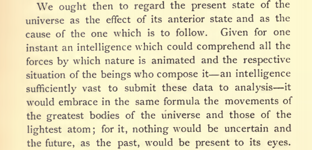
Figure: English translation of Laplace’s demon, taken from the Philosophical Essay on probabilities Laplace (1814) pg 3.

One way of viewing what Laplace is saying is that we can take “the forces by which nature is animated” or our best mathematical/computational abstraction of that which we would call the model and combine it with the “respective situation of the beings who compose it” which I would refer to as the data and if we have an “intelligence sufficiently vast enough to submit these data to analysis”, or sufficient compute then we would have a system for which “nothing would be uncertain and the future, as the past, would be present in its eyes”, or in other words we can make a prediction. Or more succinctly put we have

Laplace’s demon has been a recurring theme in science, we can also find it in Stephen Hawking’s book A Brief History of Time (A brief history of time, 1988).

If we do discover a theory of everything … it would be the ultimate triumph of human reason-for then we would truly know the mind of God

Stephen Hawking in A Brief History of Time 1988

But is it really that simple? Do we just need more and more accurate models and more and more data?

Game of Life

John Horton Conway was a mathematician who developed a game known as the Game of Life. He died in April 2020, but since he invented the game, he was in effect ‘god’ for this game. But as we will see, just inventing the rules doesn’t give you omniscience in the game.

The Game of Life is played on a grid of squares, or pixels. Each pixel is either on or off. The game has no players, but a set of simple rules that are followed at each turn the rules are.

Life Rules

John Conway’s game of life is a cellular automaton where the cells obey three very simple rules. The cells live on a rectangular grid, so that each cell has 8 possible neighbors.

loneliness

Figure: ‘Death’ through loneliness in Conway’s game of life. If a cell is surrounded by less than three cells, it ‘dies’ through loneliness.

The game proceeds in turns, and at each location in the grid is either alive or dead. Each turn, a cell counts its neighbors. If there are two or fewer neighbors, the cell ‘dies’ of ‘loneliness’.

overcrowding

Figure: ‘Death’ through overpopulation in Conway’s game of life. If a cell is surrounded by more than three cells, it ‘dies’ through loneliness.

If there are four or more neighbors, the cell ‘dies’ from ‘overcrowding’. If there are three neighbors, the cell persists, or if it is currently dead, a new cell is born.

birth

Figure: Birth in Conway’s life. Any position surrounded by precisely three live cells will give birth to a new cell at the next turn.

And that’s it. Those are the simple ‘physical laws’ for Conway’s game.

The game leads to patterns emerging, some of these patterns are static, but some oscillate in place, with varying periods. Others oscillate, but when they complete their cycle they’ve translated to a new location, in other words they move. In Life the former are known as oscillators and the latter as spaceships.

Loafers and Gliders

John Horton Conway, as the creator of the game of life, could be seen somehow as the god of this small universe. He created the rules. The rules are so simple that in many senses he, and we, are all-knowing in this space. But despite our knowledge, this world can still ‘surprise’ us. From the simple rules, emergent patterns of behaviour arise. These include static patterns that don’t change from one turn to the next. They also include, oscillators, that pulse between different forms across different periods of time. A particular form of oscillator is known as a ‘spaceship’, this is one that moves across the board as the game evolves. One of the simplest and earliest spaceships to be discovered is known as the glider.

Glider (1969)

Figure: Left A Glider pattern discovered 1969 by Richard K. Guy. Right. John Horton Conway, creator of Life (1937-2020). The glider is an oscillator that moves diagonally after creation. From the simple rules of Life it’s not obvious that such an object does exist, until you do the necessary computation.

The glider was ‘discovered’ in 1969 by Richard K. Guy. What do we mean by discovered in this context? Well, as soon as the game of life is defined, objects such as the glider do somehow exist, but the many configurations of the game mean that it takes some time for us to see one and know it exists. This means, that despite being the creator, Conway, and despite the rules of the game being simple, and despite the rules being deterministic, we are not ‘omniscient’ in any simplistic sense. It requires computation to ‘discover’ what can exist in this universe once it’s been defined.

Figure: The Gosper glider gun is a configuration that creates gliders. A new glider is released after every 30 turns.

These patterns had to be discovered, in the same way that a scientist might discover a disease, or an explorer a new land. For example, the Gosper glider gun was discovered by Bill Gosper in 1970. It is a pattern that creates a new glider every 30 turns of the game.

Despite widespread interest in Life, some of its patterns were only very recently discovered like the Loafer, discovered in 2013 by Josh Ball. So, despite the game having existed for over forty years, and the rules of the game being simple, there are emergent behaviors that are unknown.

Loafer (2013)

Figure: Left A Loafer pattern discovered by Josh Ball in 2013. Right. John Horton Conway, creator of Life (1937-2020).

Once these patterns are discovered, they are combined (or engineered) to create new Life patterns that do some remarkable things. For example, there’s a life pattern that runs a Turing machine, or more remarkably there’s a Life pattern that runs Life itself.

Figure: The Game of Life running in Life. The video is drawing out recursively showing pixels that are being formed by filling cells with moving spaceships. Each individual pixel in this game of life is made up of \(2048 \times 2048\) pixels called an OTCA metapixel.

To find out more about the Game of Life you can watch this video by Alan Zucconi or read his associated blog post.

Figure: An introduction to the Game of Life by Alan Zucconi.

Contrast this with our situation where in ‘real life’ we don’t know the simple rules of the game, the state space is larger, and emergent behaviors (hurricanes, earthquakes, volcanos, climate change) have direct consequences for our daily lives, and we understand why the process of ‘understanding’ the physical world is so difficult. We also see immediately how much easier we might expect the physical sciences to be than the social sciences, where the emergent behaviors are contingent on highly complex human interactions.

Emergent Behaviour

Laplace’s Gremlin

The curve described by a simple molecule of air or vapor is regulated in a manner just as certain as the planetary orbits; the only difference between them is that which comes from our ignorance. Probability is relative, in part to this ignorance, in part to our knowledge. We know that of three or greater number of events a single one ought to occur; but nothing induces us to believe that one of them will occur rather than the others. In this state of indecision it is impossible for us to announce their occurrence with certainty. It is, however, probable that one of these events, chosen at will, will not occur because we see several cases equally possible which exclude its occurrence, while only a single one favors it.

— Pierre-Simon Laplace (Laplace, 1814), pg 5

The representation of ignorance through probability is the true message of Laplace, I refer to this message as “Laplace’s gremlin”, because it is the gremlin of uncertainty that interferes with the demon of determinism to mean that our predictions are not deterministic.

Our separation of the uncertainty into the data, the model and the computation give us three domains in which our doubts can creep into our ability to predict. Over the last three lectures we’ve introduced some of the basic tools we can use to unpick this uncertainty. You’ve been introduced to, (or have yow reviewed) Bayes’ rule. The rule, which is a simple consequence of the product rule of probability, is the foundation of how we update our beliefs in the presence of new information.

The real point of Laplace’s essay was that we don’t have access to all the data, we don’t have access to a complete physical understanding, and as the example of the Game of Life shows, even if we did have access to both (as we do for “Conway’s universe”) we still don’t have access to all the compute that we need to make deterministic predictions. There is uncertainty in the system which means we can’t make precise predictions.

Gremlins are imaginary creatures used as an explanation of failure in aircraft, causing crashes. In that sense the Gremlin represents the uncertainty that a pilot felt about what might go wrong in a plane which might be “theoretically sound” but in practice is poorly maintained or exposed to conditions that take it beyond its design criteria. Laplace’s gremlin is all the things that your model, data and ability to compute don’t account for bringing about failures in your ability to predict. Laplace’s gremlin is the uncertainty in the system.

Figure: Gremlins are seen as the cause of a number of challenges in this World War II poster.

Abstraction and Emergent Properties

Figure: A scale of different simulations we might be interested in when modelling the physical world. The scale is \(\log_{10}\) meters. The scale reflects something about the level of granularity where we might choose to know “all positions of all items of which nature is composed”.

Unfortunately, even if such an equation were to exist, we would be unlikely to know “all positions of all items of which nature is composed”. A good example here is computational systems biology. In that domain we are interested in understanding the underlying function of the cell. These systems sit somewhere between the two extremes that Laplace described: “the movements of the greatest bodies of the universe and those of the smallest atom”.

When the smallest atom is considered, we need to introduce uncertainty. We again turn to a different work of Maxwell, building on Bernoulli’s kinetic theory of gases we end up with probabilities for representing the location of the ‘molecules of air’. Instead of a deterministic location for these particles we represent our belief about their location in a distribution.

Computational systems biology is a world of micro-machines, built of three dimensional foldings of strings of proteins. There are spindles (stators) and rotors (e.g. ATP Synthase), there are small copying machines (e.g. RNA Polymerase) there are sequence to sequence translators (Ribosomes). The cells store information in DNA but have an ecosystem of structures and messages being built and sent in proteins and RNA. Unpicking these structures has been a major preoccupation of biology. That is knowing where the atoms of these molecules are in the structure, and how the parts of the structure move when these small micro-machines are carrying out their roles.

We understand most (if not all) of the physical laws that drive the movements of these molecules, but we don’t understand all the actions of the cell, nor can we intervene reliably to improve things. So, even in the case where we have a good understanding of the physical laws, Laplace’s gremlin emerges in our knowledge of “the positions of all items of which nature is composed”.

Molecular Dynamics Simulations

By understanding and simulating the physics, we can recreate operations that are happening at the level of proteins in the human cell. V-ATPase is an enzyme that pumps protons. But at the microscopic level it’s a small machine. It produces ATP in response to a proton gradient. A paper in Science Advances (Roh et al., 2020) simulates the functioning of these proteins that operate across the cell membrane. This makes these proteins difficult to crystallize, the response to this challenge is to use a simulation which (somewhat) abstracts the processes. You can also check this blog post from the paper’s press release.

Figure: The V-ATPase enzyme pumps proteins across membranes. This molecular dynamics simulation was published in Science Advances (Roh et al., 2020). The scale is roughly \(10^{-8} m\).

Quantum Mechanics

Alternatively, we can drop down a few scales and consider simulation of the Schrödinger equation. Intractabilities in the many-electron Schrödinger equation have been addressed using deep neural networks to speed up the solution enabling simulation of chemical bonds (Pfau et al., 2020). The PR-blog post is also available. The paper uses a neural network to model the quantum state of a number of electrons.

Figure: The many-electron Schrödinger equation is important in understanding how Chemical bonds are formed.

Each of these simulations have the same property of being based on a set of (physical) rules about how particles interact. But one of the interesting characteristics of such systems is how the properties of the system are emergent as the dynamics are allowed to continue.

These properties cannot be predicted without running the physics, or the equivalently the equation. Computation is required. And often the amount of computation that is required is prohibitive.

Lenox Globe

Figure: The Lenox globe, which dates from early 16th century, one of the earliest known globes.

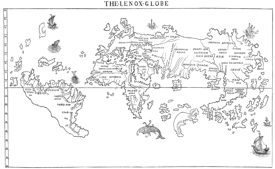
Figure: Drawing of the Lenox Globe by the historian for the Magazine of American History in September 1879.

Figure: Detail from the Lenox globe located in the region of China, “hic sunt dracones”

Weather

So what’s going on here? One analogy I like to use is with weather forecasting. Historically, before the use of computer driven weather forecasting, we used a process of interpolation to measure the pressure.

Figure: Forecast from UK Met Office on 5th June 1944. (detail from https://www.metoffice.gov.uk/research/library-and-archive/archive-hidden-treasures/d-day)

This was problematic for German forces in the Second World War because they had no ability to predict the weather when it was coming in from across the UK. Conversely, the UK had a number of weather stations in the UK, and some information (perhaps from spies or Enigma decrypts) about weather on the mainland.

Figure: Forecast from Deutscher Wetterdienst on 5th June 1944. (detail from https://www.metoffice.gov.uk/research/library-and-archive/archive-hidden-treasures/d-day). Note the lack of measurements within the UK. THis is the direction that weather was coming from so the locaiton of weather fronts (and associated storms) was harder for the Deutscher Wetterdienst to predict than the Met Office.

This meant that more accurate forecasts were possible for D-Day for the Allies than for the defending forces. As a result, on the morning that Eisenhower invated, Rommel was back in Germany attending his wife’s 50th birthday party.

Modern artificial intelligence solutions are using very large amounts of data to build a landscape in which this interpolation can take place. Tools like ChatGPT are allowing us to interpolate between different human concepts. This is an amazing achievement, but it is also a challenge.

Boulton and Watt’s Lap Engine

Lap Engine (1788)

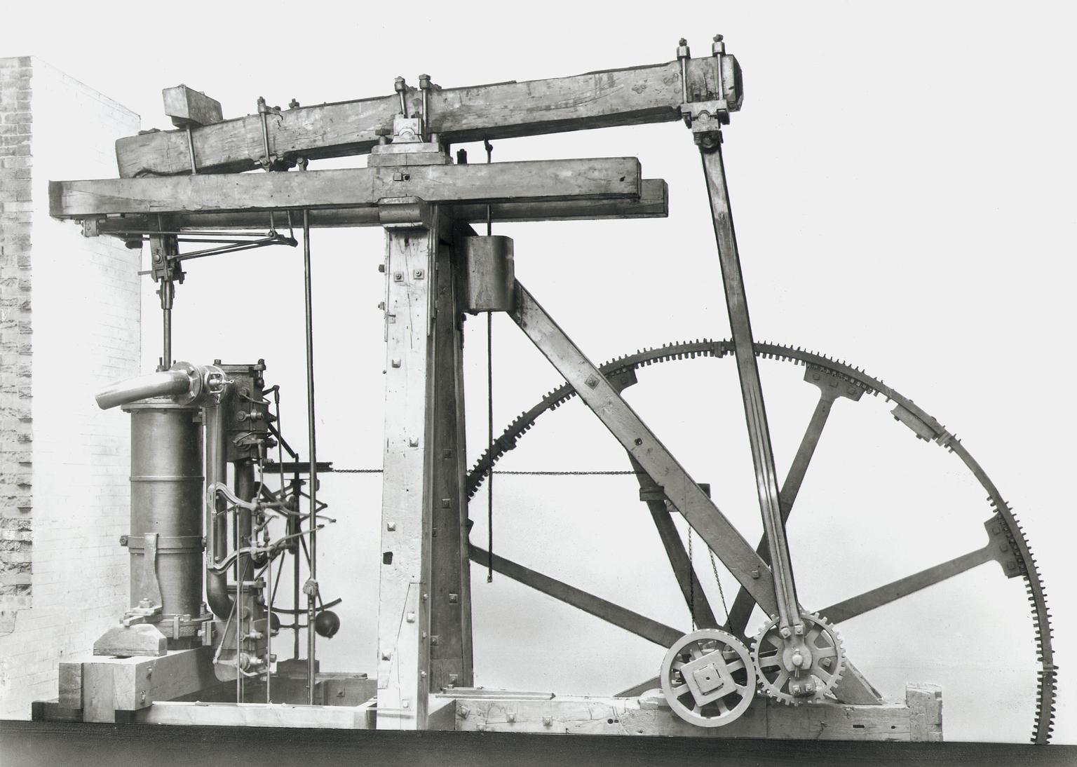
total energy = available energy + temperature \(\times\) entropy

Figure: James Watt’s Lap Engine which incorporates many of his innovations to the steam engine, making it more efficient.

Brownian Motion and Wiener

Robert Brown was a botanist who was studying plant pollen in 1827 when he noticed a trembling motion of very small particles contained within cavities within the pollen. He worked hard to eliminate the potential source of the movement by exploring other materials where he found it to be continuously present. Thus, the movement was not associated, as he originally thought, with life.

In 1905 Albert Einstein produced the first mathematical explanation of the phenomenon. This can be seen as our first model of a ‘curve of a simple molecule of air’. To model the phenomenon Einstein introduced stochasticity to a differential equation. The particles were being peppered with high-speed water molecules, that was triggering the motion. Einstein modelled this as a stochastic process.

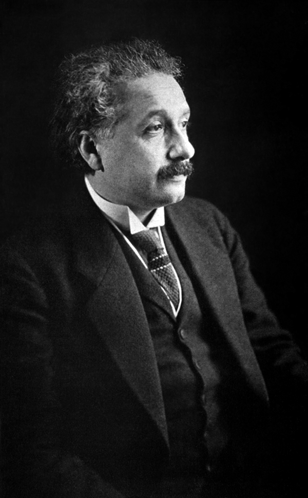
Figure: Albert Einstein’s 1905 paper on Brownian motion introduced stochastic differential equations which can be used to model the ‘curve of a simple molecule of air’.

Norbert Wiener was a child prodigy, whose father had schooled him in philosophy. He was keen to have his son work with the leading philosophers of the age, so at the age of 18 Wiener arrived in Cambridge (already with a PhD). He was despatched to study with Bertrand Russell but Wiener and Russell didn’t get along. Wiener wasn’t persuaded by Russell’s ideas for theories of knowledge through logic. He was more aligned with Laplace and his desire for a theory of ignorance. In is autobiography he relates it as the first thing he could see his father was proud of (at around the age of 10 or 11) (Wiener, 1953).

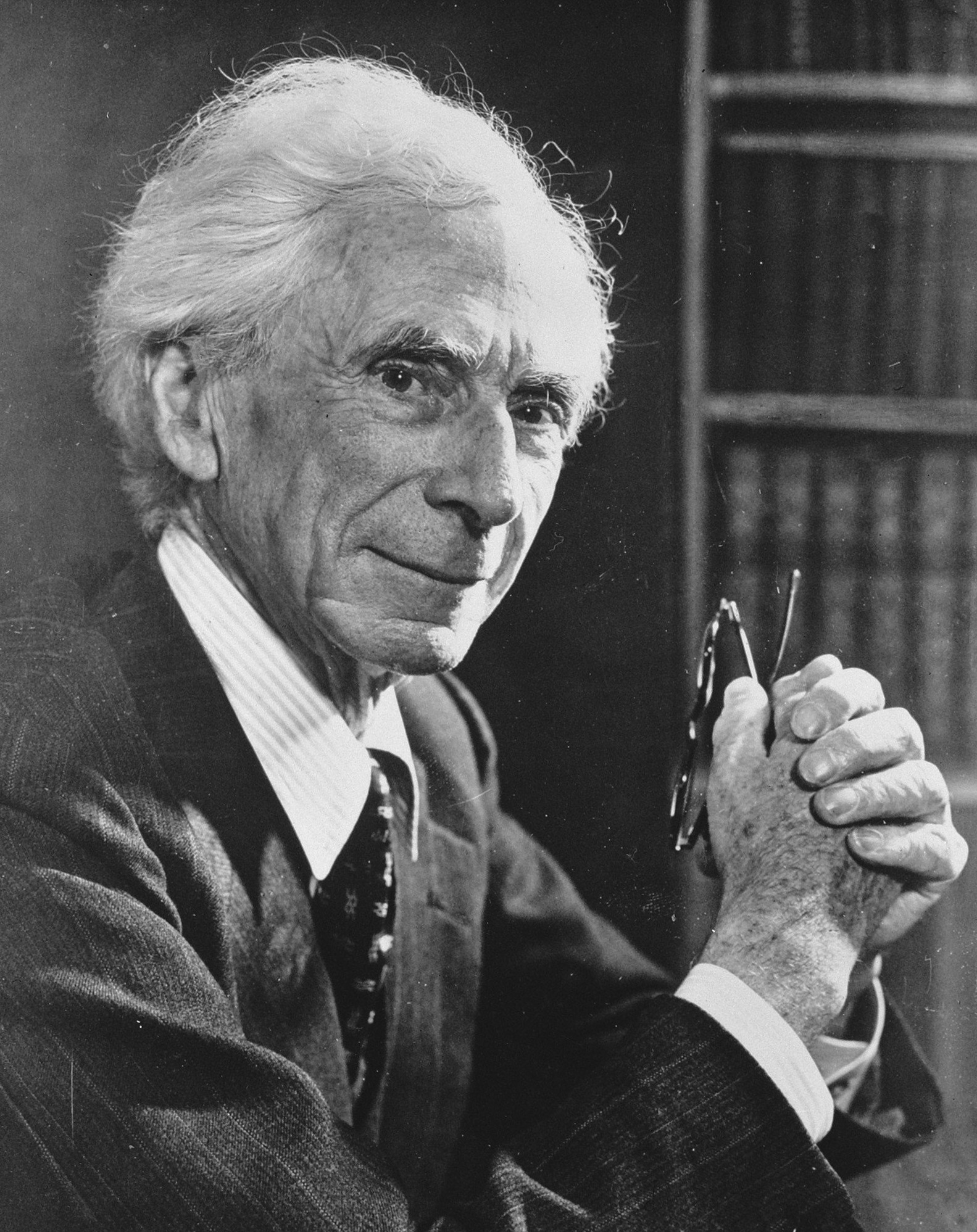
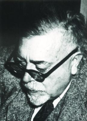
Figure: Bertrand Russell (1872-1970), Albert Einstein (1879-1955), Norbert Wiener, (1894-1964)

But Russell (despite also not getting along well with Wiener) introduced Wiener to Einstein’s works, and Wiener also met G. H. Hardy. He left Cambridge for Göttingen where he studied with Hilbert. He developed the underlying mathematics for proving the existence of the solutions to Einstein’s equation, which are now known as Wiener processes.

Figure: Brownian motion of a large particle in a group of smaller particles. The movement is known as a Wiener process after Norbert Wiener.

Figure: Norbert Wiener (1894 - 1964). Founder of cybernetics and the information era. He used Gibbs’s ideas to develop a “theory of ignorance” that he deployed in early communication. On the right is Wiener’s wartime report that used stochastic processes in forecasting with applications in radar control (image from Coales and Kane (2014)).

Wiener himself used the processes in his work. He was focused on mathematical theories of communication. Between the world wars he was based at Massachusetts Institute of Technology where the burgeoning theory of electrical engineering was emerging, with a particular focus on communication lines. Winer developed theories of communication that used Gibbs’s entropy to encode information. He also used the ideas behind the Wiener process for developing tracking methods for radar systems in the second world war. These processes are what we know of now as Gaussian processes (Wiener (1949)).

James Clerk Maxwell

Ludwig Boltzmann

Josiah Willard Gibbs

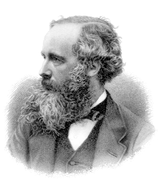
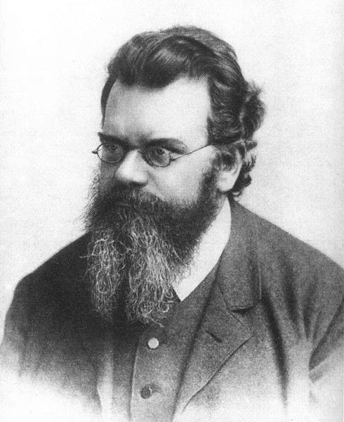
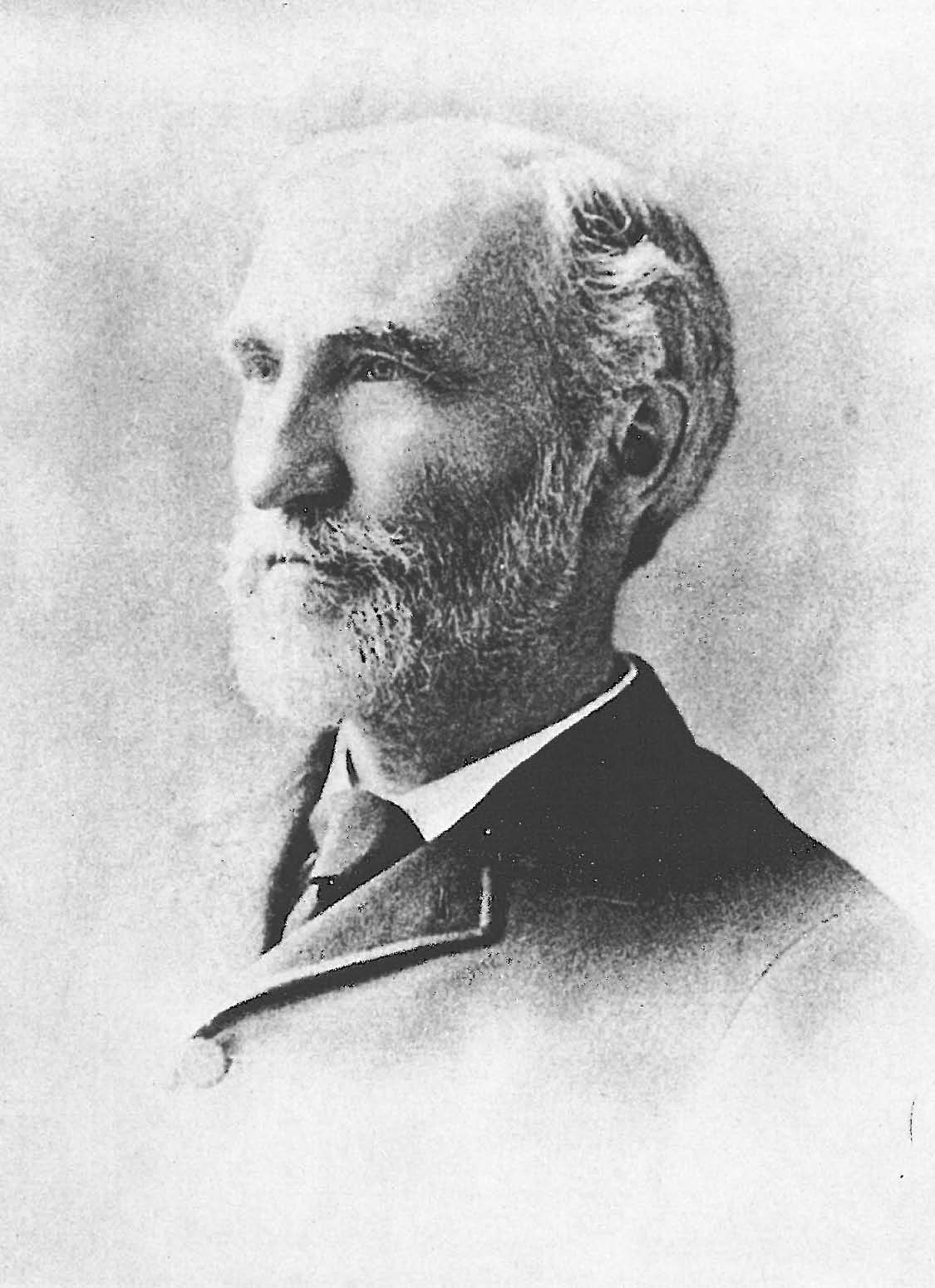
Figure: James Clerk Maxwell (1831-1879), Ludwig Boltzmann (1844-1906) Josiah Willard Gibbs (1839-1903)

Entropy Billiards

Entropy:

New Ball Pause Skip 1000s Histogram

Figure: Bernoulli’s simple kinetic models of gases assume that the molecules of air operate like billiard balls.

import numpy as np

p = np.random.randn(10000, 1)
xlim = [-4, 4]
x = np.linspace(xlim[0], xlim[1], 200)
y = 1/np.sqrt(2*np.pi)*np.exp(-0.5*x*x)

Another important figure for Cambridge was the first to derive the probability distribution that results from small balls banging together in this manner. In doing so, James Clerk Maxwell founded the field of statistical physics.

Figure: James Clerk Maxwell 1831-1879 Derived distribution of velocities of particles in an ideal gas (elastic fluid).

Maxwell’s Demon

Figure: Maxwell’s demon opens and closes a door which allows fast particles to pass from left to right and slow particles to pass from right to left. This makes the left hand side colder than the right.

Entropy:

New Ball Pause Skip 1000s Histogram

Figure: Maxwell’s Demon. The demon decides balls are either cold (blue) or hot (red) according to their velocity. Balls are allowed to pass the green membrane from right to left only if they are cold, and from left to right, only if they are hot.

Figure: Rabbit and Pooh watch the result of Pooh’s hooshing idea to move Eeyore towards the shore.

When you are a Bear of Very Little Brain, and you Think of Things, you find sometimes that a Thing which seemed very Thingish inside you is quite different when it gets out into the open and has other people looking at it.

A.A. Milne as Winnie-the-Pooh in The House at Pooh Corner, 1928

This comment from Pooh bear comes just as he’s tried to rescue his donkey friend, Eeyore, from a river by dropping a large stone on him from a bridge. Pooh’s idea had been to create a wave to push the donkey to the shore, a process that Pooh’s rabbit friend calls “hooshing”.

Hooshing is a technique many children will have tried to retrieve a ball from a river. It can work, so Pooh’s idea wasn’t a bad one, but the challenge he faced was in its execution. Pooh aimed to the side of Eeyore, unfortunately the stone fell directly on the stuffed donkey. But where is Laplace’s demon in hooshing? Just as we can talk about Gliders and Loafers in Conway’s Game of Life, we talk about stones and donkeys in our Universe. Pooh’s prediction that he can hoosh the donkey with the stone is not based on the Theory, it comes from observing the way objects interact in the actual Universe. Pooh is like the mice in Douglas Adams’s Earth. He is observing his environment. He looks for patterns in that environment. Pooh then borrows the computation that the Universe has already done for us. He has seen similar situations before, perhaps he once used a stone to hoosh a ball. He is then generalising from these previous circumstances to suggest that he can also hoosh the donkey. Despite being a bear of little brain, like the mice on Adams’s Earth, Pooh can answer questions about his universe by observing the results of the Theory of Everything playing out around him.

What is Machine Learning?

What is machine learning? At its most basic level machine learning is a combination of

\[\text{data} + \text{model} \stackrel{\text{compute}}{\rightarrow} \text{prediction}\]

where data is our observations. They can be actively or passively acquired (meta-data). The model contains our assumptions, based on previous experience. That experience can be other data, it can come from transfer learning, or it can merely be our beliefs about the regularities of the universe. In humans our models include our inductive biases. The prediction is an action to be taken or a categorization or a quality score. The reason that machine learning has become a mainstay of artificial intelligence is the importance of predictions in artificial intelligence. The data and the model are combined through computation.

In practice we normally perform machine learning using two functions. To combine data with a model we typically make use of:

a prediction function it is used to make the predictions. It includes our beliefs about the regularities of the universe, our assumptions about how the world works, e.g., smoothness, spatial similarities, temporal similarities.

an objective function it defines the ‘cost’ of misprediction. Typically, it includes knowledge about the world’s generating processes (probabilistic objectives) or the costs we pay for mispredictions (empirical risk minimization).

The combination of data and model through the prediction function and the objective function leads to a learning algorithm. The class of prediction functions and objective functions we can make use of is restricted by the algorithms they lead to. If the prediction function or the objective function are too complex, then it can be difficult to find an appropriate learning algorithm. Much of the academic field of machine learning is the quest for new learning algorithms that allow us to bring different types of models and data together.

You can also check my post blog post on What is Machine Learning?.

Kappenball

Score:

Energy:

New Ball Pause

Figure: Kappen Ball

If you want to complete a task, should you do it now or should you put it off until tomorrow? Despite being told to not delay tasks, many of us are deadline driven. Why is this?

Kappenball is a simple game that illustrates that this behaviour can be optimal. It is inspired by an example in stochastic optimal control by Bert Kappen. The game is as follows: you need to place a falling balloon into one of two holes, but if the balloon misses the holes it will pop on pins placed in the ground. In ‘deterministic mode’, the balloon falls straight towards the ground and the game is easy. You simply choose which hole to place the ball in, and you can start to place it there as soon as the ball appears at the top of the screen. The game becomes more interesting as you increase the uncertainty. In Kappenball, the uncertainty takes the form of the balloon being blown left and right as it falls. This movement means that it is not sensible to decide early on which hole to place the balloon in. A better strategy is to wait and see which hole the ball falls towards. You can then place it in that hole using less energy than in deterministic mode. Sometimes, the ball even falls into the hole on its own, and you don’t have to expend any energy, but it requires some skill to judge when you need to intervene. For this system Bert Kappen has shown mathematically that the best solution is to wait until the ball is close to the hole before you push it in. In other words, you should be deadline driven.

In fact, it seems here uncertainty is a good thing, because on average you’ll get the ball into the hole with less energy (by playing intelligently, and being deadline driven!) than you do with `deterministic mode’. It requires some skill to do this, more than the deterministic system, but by using your resources intelligently you can get more out of the system. However, if the uncertainty increases too much then regardless of your skill, you can’t control the ball at all.

This simple game explains many of the behaviours we exhibit in real life. If a system is completely deterministic, then we can make a decision early on and be sure that the ball will ‘drop in the hole’. However, if there is uncertainty in a system, it can make sense to delay our decision making until we’ve seen how events ‘pan out’. Be careful though, as we also see that when the uncertainty is large, if you don’t have the resources or the skill to be deadline-driven the uncertainty can overwhelm you and events can quickly move beyond our control.

Prime Air

One project where the components of machine learning and the physical world come together is Amazon’s Prime Air drone delivery system.

Automating the process of moving physical goods through autonomous vehicles completes the loop between the ‘bits’ and the ‘atoms’. In other words, the information and the ‘stuff’. The idea of the drone is to complete a component of package delivery, the notion of last mile movement of goods, but in a fully autonomous way.

Figure: An actual ‘Santa’s sleigh’. Amazon’s prototype delivery drone. Machine learning algorithms are used across various systems including sensing (computer vision for detection of wires, people, dogs etc) and piloting. The technology is necessarily a combination of old and new ideas. The transition from vertical to horizontal flight is vital for efficiency and uses sophisticated machine learning to achieve.

As Jeff Wilke (who was CEO of Amazon Retail at the time) announced in June 2019 the technology is ready, but still needs operationalization including e.g. regulatory approval.

Figure: Jeff Wilke (CEO Amazon Consumer) announcing the new drone at the Amazon 2019 re:MARS event alongside the scale of the Amazon supply chain.

When we announced earlier this year that we were evolving our Prime two-day shipping offer in the U.S. to a one-day program, the response was terrific. But we know customers are always looking for something better, more convenient, and there may be times when one-day delivery may not be the right choice. Can we deliver packages to customers even faster? We think the answer is yes, and one way we’re pursuing that goal is by pioneering autonomous drone technology.

Today at Amazon’s re:MARS Conference (Machine Learning, Automation, Robotics and Space) in Las Vegas, we unveiled our latest Prime Air drone design. We’ve been hard at work building fully electric drones that can fly up to 15 miles and deliver packages under five pounds to customers in less than 30 minutes. And, with the help of our world-class fulfillment and delivery network, we expect to scale Prime Air both quickly and efficiently, delivering packages via drone to customers within months.

The 15 miles in less than 30 minutes implies air speed velocities of around 50 kilometers per hour.

Our newest drone design includes advances in efficiency, stability and, most importantly, in safety. It is also unique, and it advances the state of the art. How so? First, it’s a hybrid design. It can do vertical takeoffs and landings – like a helicopter. And it’s efficient and aerodynamic—like an airplane. It also easily transitions between these two modes—from vertical-mode to airplane mode, and back to vertical mode.

It’s fully shrouded for safety. The shrouds are also the wings, which makes it efficient in flight.

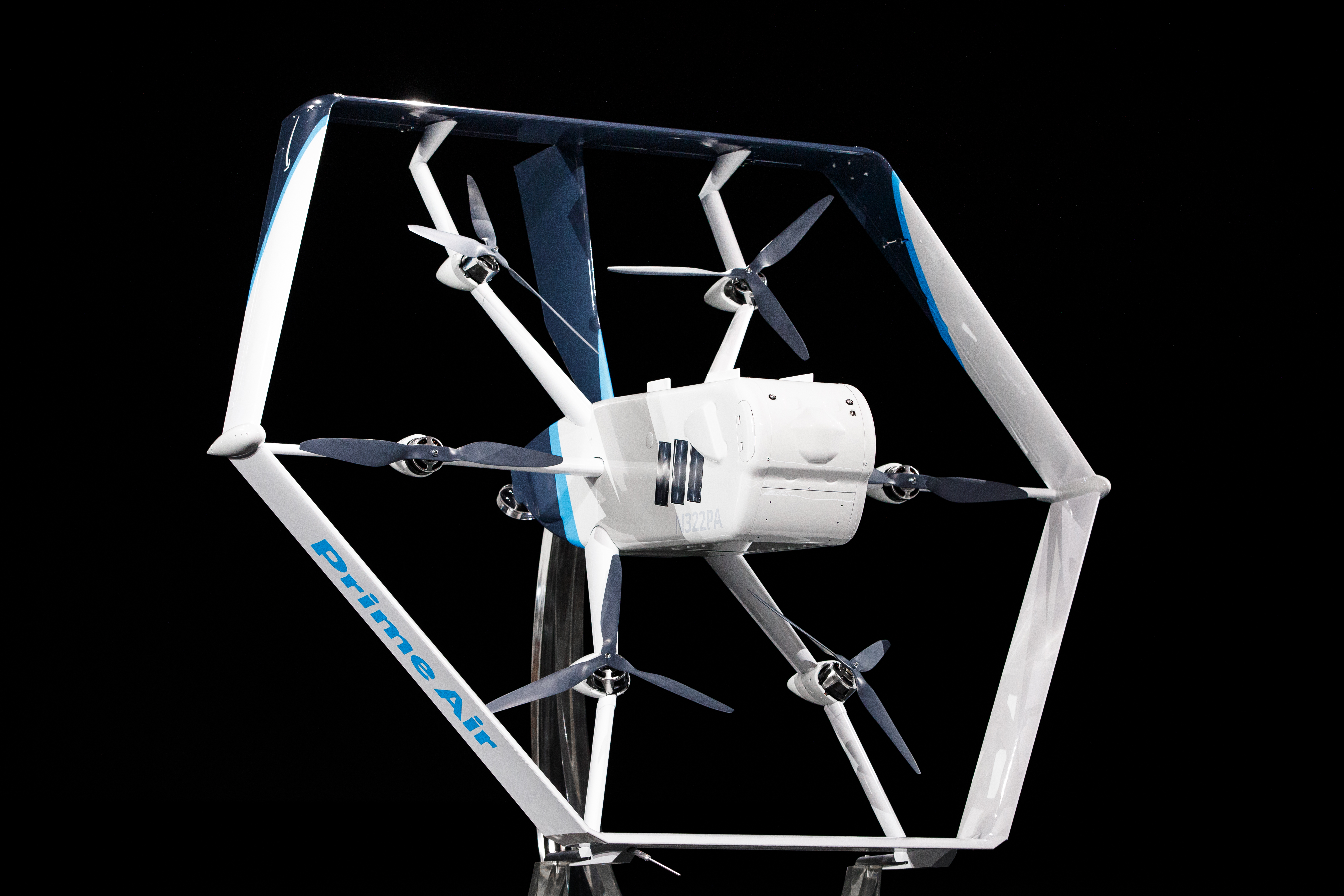
Figure: Picture of the drone from Amazon Re-MARS event in 2019.

Our drones need to be able to identify static and moving objects coming from any direction. We employ diverse sensors and advanced algorithms, such as multi-view stereo vision, to detect static objects like a chimney. To detect moving objects, like a paraglider or helicopter, we use proprietary computer-vision and machine learning algorithms.

A customer’s yard may have clotheslines, telephone wires, or electrical wires. Wire detection is one of the hardest challenges for low-altitude flights. Through the use of computer-vision techniques we’ve invented, our drones can recognize and avoid wires as they descend into, and ascend out of, a customer’s yard.

Bayesian Inference by Rejection Sampling

One view of Bayesian inference is to assume we are given a mechanism for generating samples, where we assume that mechanism is representing an accurate view on the way we believe the world works.

This mechanism is known as our prior belief.

We combine our prior belief with our observations of the real world by discarding all those prior samples that are inconsistent with our observations. The likelihood defines mathematically what we mean by inconsistent with the observations. The higher the noise level in the likelihood, the looser the notion of consistent.

The samples that remain are samples from the posterior.

This approach to Bayesian inference is closely related to two sampling techniques known as rejection sampling and importance sampling. It is realized in practice in an approach known as approximate Bayesian computation (ABC) or likelihood-free inference.

In practice, the algorithm is often too slow to be practical, because most samples will be inconsistent with the observations and as a result the mechanism must be operated many times to obtain a few posterior samples.

However, in the Gaussian process case, when the likelihood also assumes Gaussian noise, we can operate this mechanism mathematically, and obtain the posterior density analytically. This is the benefit of Gaussian processes.

First, we will load in two python functions for computing the covariance function.

Next, we sample from a multivariate normal density (a multivariate Gaussian), using the covariance function as the covariance matrix.

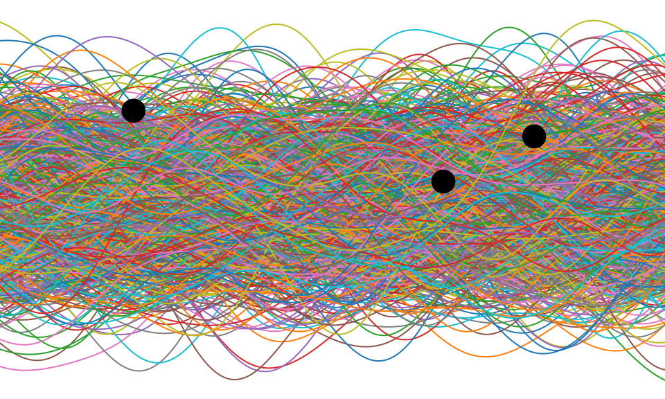
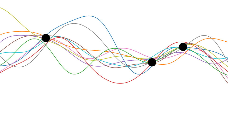
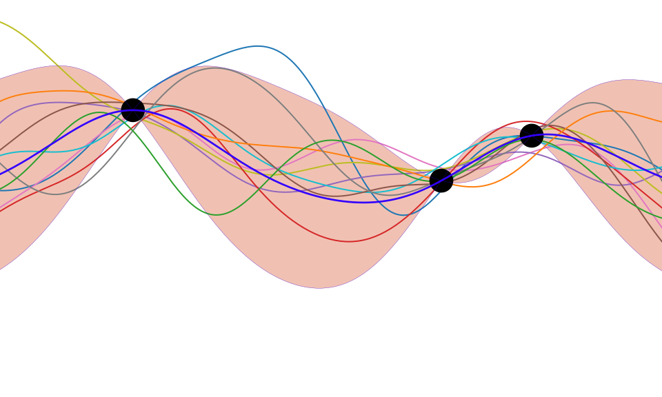
Figure: One view of Bayesian inference is we have a machine for generating samples (the prior), and we discard all samples inconsistent with our data, leaving the samples of interest (the posterior). This is a rejection sampling view of Bayesian inference. The Gaussian process allows us to do this analytically by multiplying the prior by the likelihood.

DeepFace

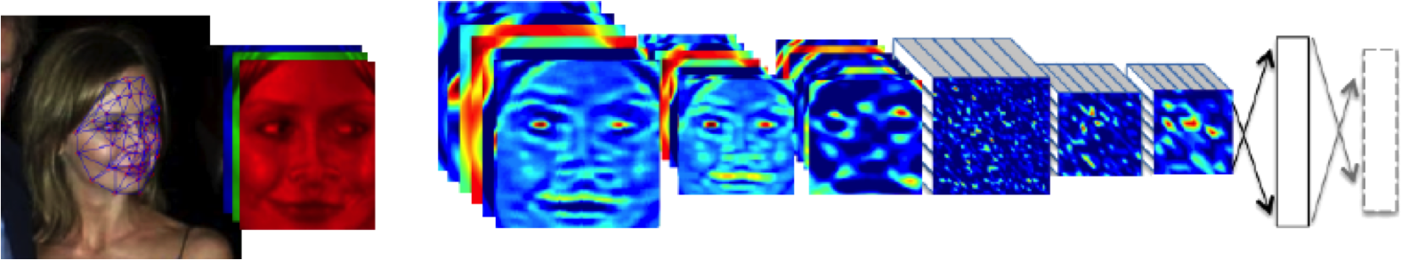
Figure: The DeepFace architecture (Taigman et al., 2014), visualized through colors to represent the functional mappings at each layer. There are 120 million parameters in the model.

The DeepFace architecture (Taigman et al., 2014) consists of layers that deal with translation invariances, known as convolutional layers. These layers are followed by three locally-connected layers and two fully-connected layers. Color illustrates feature maps produced at each layer. The neural network includes more than 120 million parameters, where more than 95% come from the local and fully connected layers.

Deep Learning as Pinball

Figure: Deep learning models are composition of simple functions. We can think of a pinball machine as an analogy. Each layer of pins corresponds to one of the layers of functions in the model. Input data is represented by the location of the ball from left to right when it is dropped in from the top. Output class comes from the position of the ball as it leaves the pins at the bottom.

Sometimes deep learning models are described as being like the brain, or too complex to understand, but one analogy I find useful to help the gist of these models is to think of them as being similar to early pin ball machines.

In a deep neural network, we input a number (or numbers), whereas in pinball, we input a ball.

Think of the location of the ball on the left-right axis as a single number. Our simple pinball machine can only take one number at a time. As the ball falls through the machine, each layer of pins can be thought of as a different layer of ‘neurons’. Each layer acts to move the ball from left to right.

In a pinball machine, when the ball gets to the bottom it might fall into a hole defining a score, in a neural network, that is equivalent to the decision: a classification of the input object.

An image has more than one number associated with it, so it is like playing pinball in a hyper-space.

Figure: At initialization, the pins, which represent the parameters of the function, aren’t in the right place to bring the balls to the correct decisions.

Figure: After learning the pins are now in the right place to bring the balls to the correct decisions.

Learning involves moving all the pins to be in the correct position, so that the ball ends up in the right place when it’s fallen through the machine. But moving all these pins in hyperspace can be difficult.

In a hyper-space you have to put a lot of data through the machine for to explore the positions of all the pins. Even when you feed many millions of data points through the machine, there are likely to be regions in the hyper-space where no ball has passed. When future test data passes through the machine in a new route unusual things can happen.

Adversarial examples exploit this high dimensional space. If you have access to the pinball machine, you can use gradient methods to find a position for the ball in the hyper space where the image looks like one thing, but will be classified as another.

Probabilistic methods explore more of the space by considering a range of possible paths for the ball through the machine. This helps to make them more data efficient and gives some robustness to adversarial examples.

Deep Neural Network

%pip install daft

Figure: A deep neural network. Input nodes are shown at the bottom. Each hidden layer is the result of applying an affine transformation to the previous layer and placing through an activation function.

Mathematically, each layer of a neural network is given through computing the activation function, \(\phi(\cdot)\), contingent on the previous layer, or the inputs. In this way the activation functions, are composed to generate more complex interactions than would be possible with any single layer. \[ \begin{align*} \mathbf{ h}_{1} &= \phi\left(\mathbf{W}_1 \mathbf{ x}\right)\\ \mathbf{ h}_{2} &= \phi\left(\mathbf{W}_2\mathbf{ h}_{1}\right)\\ \mathbf{ h}_{3} &= \phi\left(\mathbf{W}_3 \mathbf{ h}_{2}\right)\\ f&= \mathbf{ w}_4 ^\top\mathbf{ h}_{3} \end{align*} \]

Bottleneck Layers in Deep Neural Networks

Figure: Inserting the bottleneck layers introduces a new set of variables.

Including the low rank decomposition of \(\mathbf{W}\) in the neural network, we obtain a new mathematical form. Effectively, we are adding additional latent layers, \(\mathbf{ z}\), in between each of the existing hidden layers. In a neural network these are sometimes known as bottleneck layers. The network can now be written mathematically as \[ \begin{align} \mathbf{ z}_{1} &= \mathbf{V}^\top_1 \mathbf{ x}\\ \mathbf{ h}_{1} &= \phi\left(\mathbf{U}_1 \mathbf{ z}_{1}\right)\\ \mathbf{ z}_{2} &= \mathbf{V}^\top_2 \mathbf{ h}_{1}\\ \mathbf{ h}_{2} &= \phi\left(\mathbf{U}_2 \mathbf{ z}_{2}\right)\\ \mathbf{ z}_{3} &= \mathbf{V}^\top_3 \mathbf{ h}_{2}\\ \mathbf{ h}_{3} &= \phi\left(\mathbf{U}_3 \mathbf{ z}_{3}\right)\\ \mathbf{ y}&= \mathbf{ w}_4^\top\mathbf{ h}_{3}. \end{align} \]

\[ \begin{align} \mathbf{ z}_{1} &= \mathbf{V}^\top_1 \mathbf{ x}\\ \mathbf{ z}_{2} &= \mathbf{V}^\top_2 \phi\left(\mathbf{U}_1 \mathbf{ z}_{1}\right)\\ \mathbf{ z}_{3} &= \mathbf{V}^\top_3 \phi\left(\mathbf{U}_2 \mathbf{ z}_{2}\right)\\ \mathbf{ y}&= \mathbf{ w}_4 ^\top \mathbf{ z}_{3} \end{align} \]

Cascade of Gaussian Processes

Now if we replace each of these neural networks with a Gaussian process. This is equivalent to taking the limit as the width of each layer goes to infinity, while appropriately scaling down the outputs.

\[ \begin{align} \mathbf{ z}_{1} &= \mathbf{ f}_1\left(\mathbf{ x}\right)\\ \mathbf{ z}_{2} &= \mathbf{ f}_2\left(\mathbf{ z}_{1}\right)\\ \mathbf{ z}_{3} &= \mathbf{ f}_3\left(\mathbf{ z}_{2}\right)\\ \mathbf{ y}&= \mathbf{ f}_4\left(\mathbf{ z}_{3}\right) \end{align} \]

%pip install gpy

GPy: A Gaussian Process Framework in Python

Gaussian processes are a flexible tool for non-parametric analysis with uncertainty. The GPy software was started in Sheffield to provide a easy to use interface to GPs. One which allowed the user to focus on the modelling rather than the mathematics.

Figure: GPy is a BSD licensed software code base for implementing Gaussian process models in Python. It is designed for teaching and modelling. We welcome contributions which can be made through the GitHub repository https://github.com/SheffieldML/GPy

GPy is a BSD licensed software code base for implementing Gaussian process models in python. This allows GPs to be combined with a wide variety of software libraries.

The software itself is available on GitHub and the team welcomes contributions.

The aim for GPy is to be a probabilistic-style programming language, i.e., you specify the model rather than the algorithm. As well as a large range of covariance functions the software allows for non-Gaussian likelihoods, multivariate outputs, dimensionality reduction and approximations for larger data sets.

The documentation for GPy can be found here.

This notebook depends on PyDeepGP. This library can be installed via pip.

%pip install --upgrade git+https://github.com/SheffieldML/PyDeepGP.git

%pip install mlai

# Late bind setup methods to DeepGP object
from mlai.deepgp_tutorial import initialize
from mlai.deepgp_tutorial import staged_optimize
from mlai.deepgp_tutorial import posterior_sample
from mlai.deepgp_tutorial import visualize
from mlai.deepgp_tutorial import visualize_pinball

import deepgp
deepgp.DeepGP.initialize=initialize
deepgp.DeepGP.staged_optimize=staged_optimize
deepgp.DeepGP.posterior_sample=posterior_sample
deepgp.DeepGP.visualize=visualize
deepgp.DeepGP.visualize_pinball=visualize_pinball

Olympic Marathon Data

Gold medal times for Olympic Marathon since 1896. Marathons before 1924 didn’t have a standardized distance. Present results using pace per km. In 1904 Marathon was badly organized leading to very slow times.

Image from Wikimedia Commons http://bit.ly/16kMKHQ

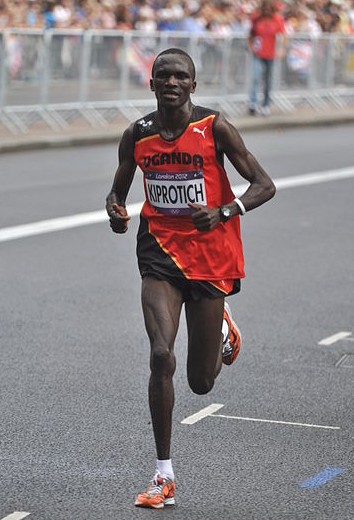
The first thing we will do is load a standard data set for regression modelling. The data consists of the pace of Olympic Gold Medal Marathon winners for the Olympics from 1896 to present. Let’s load in the data and plot.

%pip install pods

import numpy as np
import pods

data = pods.datasets.olympic_marathon_men()
x = data['X']
y = data['Y']

offset = y.mean()
scale = np.sqrt(y.var())
yhat = (y - offset)/scale

Figure: Olympic marathon pace times since 1896.

Things to notice about the data include the outlier in 1904, in that year the Olympics was in St Louis, USA. Organizational problems and challenges with dust kicked up by the cars following the race meant that participants got lost, and only very few participants completed. More recent years see more consistently quick marathons.

Alan Turing

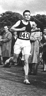
Figure: Alan Turing, in 1946 he was only 11 minutes slower than the winner of the 1948 games. Would he have won a hypothetical games held in 1946? Source: Alan Turing Internet Scrapbook.

If we had to summarise the objectives of machine learning in one word, a very good candidate for that word would be generalization. What is generalization? From a human perspective it might be summarised as the ability to take lessons learned in one domain and apply them to another domain. If we accept the definition given in the first session for machine learning, \[ \text{data} + \text{model} \stackrel{\text{compute}}{\rightarrow} \text{prediction} \] then we see that without a model we can’t generalise: we only have data. Data is fine for answering very specific questions, like “Who won the Olympic Marathon in 2012?”, because we have that answer stored, however, we are not given the answer to many other questions. For example, Alan Turing was a formidable marathon runner, in 1946 he ran a time 2 hours 46 minutes (just under four minutes per kilometer, faster than I and most of the other Endcliffe Park Run runners can do 5 km). What is the probability he would have won an Olympics if one had been held in 1946?

To answer this question we need to generalize, but before we formalize the concept of generalization let’s introduce some formal representation of what it means to generalize in machine learning.

Gaussian Process Fit

Our first objective will be to perform a Gaussian process fit to the data, we’ll do this using the GPy software.

import GPy

m_full = GPy.models.GPRegression(x,yhat)
_ = m_full.optimize() # Optimize parameters of covariance function

The first command sets up the model, then m_full.optimize() optimizes the parameters of the covariance function and the noise level of the model. Once the fit is complete, we’ll try creating some test points, and computing the output of the GP model in terms of the mean and standard deviation of the posterior functions between 1870 and 2030. We plot the mean function and the standard deviation at 200 locations. We can obtain the predictions using y_mean, y_var = m_full.predict(xt)

xt = np.linspace(1870,2030,200)[:,np.newaxis]
yt_mean, yt_var = m_full.predict(xt)
yt_sd=np.sqrt(yt_var)

Now we plot the results using the helper function in mlai.plot.

Figure: Gaussian process fit to the Olympic Marathon data. The error bars are too large, perhaps due to the outlier from 1904.

Fit Quality

In the fit we see that the error bars (coming mainly from the noise variance) are quite large. This is likely due to the outlier point in 1904, ignoring that point we can see that a tighter fit is obtained. To see this make a version of the model, m_clean, where that point is removed.

x_clean=np.vstack((x[0:2, :], x[3:, :]))
y_clean=np.vstack((yhat[0:2, :], yhat[3:, :]))

m_clean = GPy.models.GPRegression(x_clean,y_clean)
_ = m_clean.optimize()

Deep GP Fit

Let’s see if a deep Gaussian process can help here. We will construct a deep Gaussian process with one hidden layer (i.e. one Gaussian process feeding into another).

Build a Deep GP with an additional hidden layer (one dimensional) to fit the model.

import GPy
import deepgp

hidden = 1
m = deepgp.DeepGP([y.shape[1],hidden,x.shape[1]],Y=yhat, X=x, inits=['PCA','PCA'], 
                  kernels=[GPy.kern.RBF(hidden,ARD=True),
                           GPy.kern.RBF(x.shape[1],ARD=True)], # the kernels for each layer
                  num_inducing=50, back_constraint=False)

# Call the initalization
m.initialize()

Now optimize the model.

for layer in m.layers:
    layer.likelihood.variance.constrain_positive(warning=False)
m.optimize(messages=True,max_iters=10000)

m.staged_optimize(messages=(True,True,True))

Olympic Marathon Data Deep GP

Figure: Deep GP fit to the Olympic marathon data. Error bars now change as the prediction evolves.

Olympic Marathon Data Deep GP

Figure: Point samples run through the deep Gaussian process show the distribution of output locations.

Fitted GP for each layer

Now we explore the GPs the model has used to fit each layer. First of all, we look at the hidden layer.

Figure: The mapping from input to the latent layer is broadly, with some flattening as time goes on. Variance is high across the input range.

Figure: The mapping from the latent layer to the output layer.

Olympic Marathon Pinball Plot

Figure: A pinball plot shows the movement of the ‘ball’ as it passes through each layer of the Gaussian processes. Mean directions of movement are shown by lines. Shading gives one standard deviation of movement position. At each layer, the uncertainty is reset. The overal uncertainty is the cumulative uncertainty from all the layers. There is some grouping of later points towards the right in the first layer, which also injects a large amount of uncertainty. Due to flattening of the curve in the second layer towards the right the uncertainty is reduced in final output.

The pinball plot shows the flow of any input ball through the deep Gaussian process. In a pinball plot a series of vertical parallel lines would indicate a purely linear function. For the olypmic marathon data we can see the first layer begins to shift from input towards the right. Note it also does so with some uncertainty (indicated by the shaded backgrounds). The second layer has less uncertainty, but bunches the inputs more strongly to the right. This input layer of uncertainty, followed by a layer that pushes inputs to the right is what gives the heteroschedastic noise.

Step Function

Next we consider a simple step function data set.

num_low=25
num_high=25
gap = -.1
noise=0.0001
x = np.vstack((np.linspace(-1, -gap/2.0, num_low)[:, np.newaxis],
              np.linspace(gap/2.0, 1, num_high)[:, np.newaxis]))
y = np.vstack((np.zeros((num_low, 1)), np.ones((num_high,1))))
scale = np.sqrt(y.var())
offset = y.mean()
yhat = (y-offset)/scale

Step Function Data

Figure: Simulation study of step function data artificially generated. Here there is a small overlap between the two lines.

Step Function Data GP

We can fit a Gaussian process to the step function data using GPy as follows.

m_full = GPy.models.GPRegression(x,yhat)
_ = m_full.optimize() # Optimize parameters of covariance function

Where GPy.models.GPRegression() gives us a standard GP regression model with exponentiated quadratic covariance function.

The model is optimized using m_full.optimize() which calls an L-BGFS gradient based solver in python.

Figure: Gaussian process fit to the step function data. Note the large error bars and the over-smoothing of the discontinuity. Error bars are shown at two standard deviations.

The resulting fit to the step function data shows some challenges. In particular, the over smoothing at the discontinuity. If we know how many discontinuities there are, we can parameterize them in the step function. But by doing this, we form a semi-parametric model. The parameters indicate how many discontinuities are, and where they are. They can be optimized as part of the model fit. But if new, unforeseen, discontinuities arise when the model is being deployed in practice, these won’t be accounted for in the predictions.

Step Function Data Deep GP

First we initialize a deep Gaussian process with three latent layers (four layers total). Within each layer we create a GP with an exponentiated quadratic covariance (GPy.kern.RBF).

At each layer we use 20 inducing points for the variational approximation.

layers = [y.shape[1], 1, 1, 1,x.shape[1]]
inits = ['PCA']*(len(layers)-1)
kernels = []
for i in layers[1:]:
    kernels += [GPy.kern.RBF(i)]
    
m = deepgp.DeepGP(layers,Y=yhat, X=x, 
                  inits=inits, 
                  kernels=kernels, # the kernels for each layer
                  num_inducing=20, back_constraint=False)

Once the model is constructed we initialize the parameters, and perform the staged optimization which starts by optimizing variational parameters with a low noise and proceeds to optimize the whole model.

m.initialize()
m.staged_optimize()

We plot the output of the deep Gaussian process fitted to the step data as follows.

The deep Gaussian process does a much better job of fitting the data. It handles the discontinuity easily, and error bars drop to smaller values in the regions of data.

Figure: Deep Gaussian process fit to the step function data.

Step Function Data Deep GP

The samples of the model can be plotted with the helper function from mlai.plot, model_sample

The samples from the model show that the error bars, which are informative for Gaussian outputs, are less informative for this model. They make clear that the data points lie, in output mainly at 0 or 1, or occasionally in between.

Figure: Samples from the deep Gaussian process model for the step function fit.

The visualize code allows us to inspect the intermediate layers in the deep GP model to understand how it has reconstructed the step function.

Figure: From top to bottom, the Gaussian process mapping function that makes up each layer of the resulting deep Gaussian process.

A pinball plot can be created for the resulting model to understand how the input is being translated to the output across the different layers.

Figure: Pinball plot of the deep GP fitted to the step function data. Each layer of the model pushes the ‘ball’ towards the left or right, saturating at 1 and 0. This causes the final density to be be peaked at 0 and 1. Transitions occur driven by the uncertainty of the mapping in each layer.

The Future

What does this mean for the future? Although I’ve focussed mainly on uncertainty I think that the main area for future research is interaction. Coming back to dynamic systems, but not just interaction between planes and people, interactions of the form of conversation. Interventions intelligently selected rather than emulated.

Conclusions

The probabilistic modelling community has evolved in an era where the assumption was that ambiguous conclusions are best shared with a (trained) professional through probabilities. Recent advances in generative AI offer the possibility of machines that have a better understanding of human subjective ambiguities and therefore machines that can summarise information in a way that can be interogated rather than just through a series of numbers.

Thanks!

For more information on these subjects and more you might want to check the following resources.

• book: The Atomic Human
• twitter: @lawrennd
• podcast: The Talking Machines
• newspaper: Guardian Profile Page
• blog: http://inverseprobability.com

References