AI and Business

Neil D. Lawrence

$$\newcommand{\tk}[1]{} \newcommand{\Amatrix}{\mathbf{A}} \newcommand{\KL}[2]{\text{KL}\left( #1\,\|\,#2 \right)} \newcommand{\Kaast}{\kernelMatrix_{\mathbf{ \ast}\mathbf{ \ast}}} \newcommand{\Kastu}{\kernelMatrix_{\mathbf{ \ast} \inducingVector}} \newcommand{\Kff}{\kernelMatrix_{\mappingFunctionVector \mappingFunctionVector}} \newcommand{\Kfu}{\kernelMatrix_{\mappingFunctionVector \inducingVector}} \newcommand{\Kuast}{\kernelMatrix_{\inducingVector \bf\ast}} \newcommand{\Kuf}{\kernelMatrix_{\inducingVector \mappingFunctionVector}} \newcommand{\Kuu}{\kernelMatrix_{\inducingVector \inducingVector}} \newcommand{\Kuui}{\Kuu^{-1}} \newcommand{\Qaast}{\mathbf{Q}_{\bf \ast \ast}} \newcommand{\Qastf}{\mathbf{Q}_{\ast \mappingFunction}} \newcommand{\Qfast}{\mathbf{Q}_{\mappingFunctionVector \bf \ast}} \newcommand{\Qff}{\mathbf{Q}_{\mappingFunctionVector \mappingFunctionVector}} \newcommand{\aMatrix}{\mathbf{A}} \newcommand{\aScalar}{a} \newcommand{\aVector}{\mathbf{a}} \newcommand{\acceleration}{a} \newcommand{\bMatrix}{\mathbf{B}} \newcommand{\bScalar}{b} \newcommand{\bVector}{\mathbf{b}} \newcommand{\basisFunc}{\phi} \newcommand{\basisFuncVector}{\boldsymbol{ \basisFunc}} \newcommand{\basisFunction}{\phi} \newcommand{\basisLocation}{\mu} \newcommand{\basisMatrix}{\boldsymbol{ \Phi}} \newcommand{\basisScalar}{\basisFunction} \newcommand{\basisVector}{\boldsymbol{ \basisFunction}} \newcommand{\activationFunction}{\phi} \newcommand{\activationMatrix}{\boldsymbol{ \Phi}} \newcommand{\activationScalar}{\basisFunction} \newcommand{\activationVector}{\boldsymbol{ \basisFunction}} \newcommand{\bigO}{\mathcal{O}} \newcommand{\binomProb}{\pi} \newcommand{\cMatrix}{\mathbf{C}} \newcommand{\cbasisMatrix}{\hat{\boldsymbol{ \Phi}}} \newcommand{\cdataMatrix}{\hat{\dataMatrix}} \newcommand{\cdataScalar}{\hat{\dataScalar}} \newcommand{\cdataVector}{\hat{\dataVector}} \newcommand{\centeredKernelMatrix}{\mathbf{ \MakeUppercase{\centeredKernelScalar}}} \newcommand{\centeredKernelScalar}{b} \newcommand{\centeredKernelVector}{\centeredKernelScalar} \newcommand{\centeringMatrix}{\mathbf{H}} \newcommand{\chiSquaredDist}[2]{\chi_{#1}^{2}\left(#2\right)} \newcommand{\chiSquaredSamp}[1]{\chi_{#1}^{2}} \newcommand{\conditionalCovariance}{\boldsymbol{ \Sigma}} \newcommand{\coregionalizationMatrix}{\mathbf{B}} \newcommand{\coregionalizationScalar}{b} \newcommand{\coregionalizationVector}{\mathbf{ \coregionalizationScalar}} \newcommand{\covDist}[2]{\text{cov}_{#2}\left(#1\right)} \newcommand{\covSamp}[1]{\text{cov}\left(#1\right)} \newcommand{\covarianceScalar}{c} \newcommand{\covarianceVector}{\mathbf{ \covarianceScalar}} \newcommand{\covarianceMatrix}{\mathbf{C}} \newcommand{\covarianceMatrixTwo}{\boldsymbol{ \Sigma}} \newcommand{\croupierScalar}{s} \newcommand{\croupierVector}{\mathbf{ \croupierScalar}} \newcommand{\croupierMatrix}{\mathbf{ \MakeUppercase{\croupierScalar}}} \newcommand{\dataDim}{p} \newcommand{\dataIndex}{i} \newcommand{\dataIndexTwo}{j} \newcommand{\dataMatrix}{\mathbf{Y}} \newcommand{\dataScalar}{y} \newcommand{\dataSet}{\mathcal{D}} \newcommand{\dataStd}{\sigma} \newcommand{\dataVector}{\mathbf{ \dataScalar}} \newcommand{\decayRate}{d} \newcommand{\degreeMatrix}{\mathbf{ \MakeUppercase{\degreeScalar}}} \newcommand{\degreeScalar}{d} \newcommand{\degreeVector}{\mathbf{ \degreeScalar}} \newcommand{\diag}[1]{\text{diag}\left(#1\right)} \newcommand{\diagonalMatrix}{\mathbf{D}} \newcommand{\diff}[2]{\frac{\text{d}#1}{\text{d}#2}} \newcommand{\diffTwo}[2]{\frac{\text{d}^2#1}{\text{d}#2^2}} \newcommand{\displacement}{x} \newcommand{\displacementVector}{\textbf{\displacement}} \newcommand{\distanceMatrix}{\mathbf{ \MakeUppercase{\distanceScalar}}} \newcommand{\distanceScalar}{d} \newcommand{\distanceVector}{\mathbf{ \distanceScalar}} \newcommand{\eigenvaltwo}{\ell} \newcommand{\eigenvaltwoMatrix}{\mathbf{L}} \newcommand{\eigenvaltwoVector}{\mathbf{l}} \newcommand{\eigenvalue}{\lambda} \newcommand{\eigenvalueMatrix}{\boldsymbol{ \Lambda}} \newcommand{\eigenvalueVector}{\boldsymbol{ \lambda}} \newcommand{\eigenvector}{\mathbf{ \eigenvectorScalar}} \newcommand{\eigenvectorMatrix}{\mathbf{U}} \newcommand{\eigenvectorScalar}{u} \newcommand{\eigenvectwo}{\mathbf{v}} \newcommand{\eigenvectwoMatrix}{\mathbf{V}} \newcommand{\eigenvectwoScalar}{v} \newcommand{\entropy}[1]{\mathcal{H}\left(#1\right)} \newcommand{\errorFunction}{E} \newcommand{\expDist}[2]{\left\langle#1\right\rangle_{#2}} \newcommand{\expSamp}[1]{\left\langle#1\right\rangle} \newcommand{\expectation}[1]{\left\langle #1 \right\rangle } \newcommand{\expectationDist}[2]{\left\langle #1 \right\rangle _{#2}} \newcommand{\expectedDistanceMatrix}{\mathcal{D}} \newcommand{\eye}{\mathbf{I}} \newcommand{\fantasyDim}{r} \newcommand{\fantasyMatrix}{\mathbf{ \MakeUppercase{\fantasyScalar}}} \newcommand{\fantasyScalar}{z} \newcommand{\fantasyVector}{\mathbf{ \fantasyScalar}} \newcommand{\featureStd}{\varsigma} \newcommand{\gammaCdf}[3]{\mathcal{GAMMA CDF}\left(#1|#2,#3\right)} \newcommand{\gammaDist}[3]{\mathcal{G}\left(#1|#2,#3\right)} \newcommand{\gammaSamp}[2]{\mathcal{G}\left(#1,#2\right)} \newcommand{\gaussianDist}[3]{\mathcal{N}\left(#1|#2,#3\right)} \newcommand{\gaussianSamp}[2]{\mathcal{N}\left(#1,#2\right)} \newcommand{\uniformDist}[3]{\mathcal{U}\left(#1|#2,#3\right)} \newcommand{\uniformSamp}[2]{\mathcal{U}\left(#1,#2\right)} \newcommand{\given}{|} \newcommand{\half}{\frac{1}{2}} \newcommand{\heaviside}{H} \newcommand{\hiddenMatrix}{\mathbf{ \MakeUppercase{\hiddenScalar}}} \newcommand{\hiddenScalar}{h} \newcommand{\hiddenVector}{\mathbf{ \hiddenScalar}} \newcommand{\identityMatrix}{\eye} \newcommand{\inducingInputScalar}{z} \newcommand{\inducingInputVector}{\mathbf{ \inducingInputScalar}} \newcommand{\inducingInputMatrix}{\mathbf{Z}} \newcommand{\inducingScalar}{u} \newcommand{\inducingVector}{\mathbf{ \inducingScalar}} \newcommand{\inducingMatrix}{\mathbf{U}} \newcommand{\inlineDiff}[2]{\text{d}#1/\text{d}#2} \newcommand{\inputDim}{q} \newcommand{\inputMatrix}{\mathbf{X}} \newcommand{\inputScalar}{x} \newcommand{\inputSpace}{\mathcal{X}} \newcommand{\inputVals}{\inputVector} \newcommand{\inputVector}{\mathbf{ \inputScalar}} \newcommand{\iterNum}{k} \newcommand{\kernel}{\kernelScalar} \newcommand{\kernelMatrix}{\mathbf{K}} \newcommand{\kernelScalar}{k} \newcommand{\kernelVector}{\mathbf{ \kernelScalar}} \newcommand{\kff}{\kernelScalar_{\mappingFunction \mappingFunction}} \newcommand{\kfu}{\kernelVector_{\mappingFunction \inducingScalar}} \newcommand{\kuf}{\kernelVector_{\inducingScalar \mappingFunction}} \newcommand{\kuu}{\kernelVector_{\inducingScalar \inducingScalar}} \newcommand{\lagrangeMultiplier}{\lambda} \newcommand{\lagrangeMultiplierMatrix}{\boldsymbol{ \Lambda}} \newcommand{\lagrangian}{L} \newcommand{\laplacianFactor}{\mathbf{ \MakeUppercase{\laplacianFactorScalar}}} \newcommand{\laplacianFactorScalar}{m} \newcommand{\laplacianFactorVector}{\mathbf{ \laplacianFactorScalar}} \newcommand{\laplacianMatrix}{\mathbf{L}} \newcommand{\laplacianScalar}{\ell} \newcommand{\laplacianVector}{\mathbf{ \ell}} \newcommand{\latentDim}{q} \newcommand{\latentDistanceMatrix}{\boldsymbol{ \Delta}} \newcommand{\latentDistanceScalar}{\delta} \newcommand{\latentDistanceVector}{\boldsymbol{ \delta}} \newcommand{\latentForce}{f} \newcommand{\latentFunction}{u} \newcommand{\latentFunctionVector}{\mathbf{ \latentFunction}} \newcommand{\latentFunctionMatrix}{\mathbf{ \MakeUppercase{\latentFunction}}} \newcommand{\latentIndex}{j} \newcommand{\latentScalar}{z} \newcommand{\latentVector}{\mathbf{ \latentScalar}} \newcommand{\latentMatrix}{\mathbf{Z}} \newcommand{\learnRate}{\eta} \newcommand{\lengthScale}{\ell} \newcommand{\rbfWidth}{\ell} \newcommand{\likelihoodBound}{\mathcal{L}} \newcommand{\likelihoodFunction}{L} \newcommand{\locationScalar}{\mu} \newcommand{\locationVector}{\boldsymbol{ \locationScalar}} \newcommand{\locationMatrix}{\mathbf{M}} \newcommand{\variance}[1]{\text{var}\left( #1 \right)} \newcommand{\mappingFunction}{f} \newcommand{\mappingFunctionMatrix}{\mathbf{F}} \newcommand{\mappingFunctionTwo}{g} \newcommand{\mappingFunctionTwoMatrix}{\mathbf{G}} \newcommand{\mappingFunctionTwoVector}{\mathbf{ \mappingFunctionTwo}} \newcommand{\mappingFunctionVector}{\mathbf{ \mappingFunction}} \newcommand{\scaleScalar}{s} \newcommand{\mappingScalar}{w} \newcommand{\mappingVector}{\mathbf{ \mappingScalar}} \newcommand{\mappingMatrix}{\mathbf{W}} \newcommand{\mappingScalarTwo}{v} \newcommand{\mappingVectorTwo}{\mathbf{ \mappingScalarTwo}} \newcommand{\mappingMatrixTwo}{\mathbf{V}} \newcommand{\maxIters}{K} \newcommand{\meanMatrix}{\mathbf{M}} \newcommand{\meanScalar}{\mu} \newcommand{\meanTwoMatrix}{\mathbf{M}} \newcommand{\meanTwoScalar}{m} \newcommand{\meanTwoVector}{\mathbf{ \meanTwoScalar}} \newcommand{\meanVector}{\boldsymbol{ \meanScalar}} \newcommand{\mrnaConcentration}{m} \newcommand{\naturalFrequency}{\omega} \newcommand{\neighborhood}[1]{\mathcal{N}\left( #1 \right)} \newcommand{\neilurl}{http://inverseprobability.com/} \newcommand{\noiseMatrix}{\boldsymbol{ E}} \newcommand{\noiseScalar}{\epsilon} \newcommand{\noiseVector}{\boldsymbol{ \epsilon}} \newcommand{\noiseStd}{\sigma} \newcommand{\norm}[1]{\left\Vert #1 \right\Vert} \newcommand{\normalizedLaplacianMatrix}{\hat{\mathbf{L}}} \newcommand{\normalizedLaplacianScalar}{\hat{\ell}} \newcommand{\normalizedLaplacianVector}{\hat{\mathbf{ \ell}}} \newcommand{\numActive}{m} \newcommand{\numBasisFunc}{m} \newcommand{\numComponents}{m} \newcommand{\numComps}{K} \newcommand{\numData}{n} \newcommand{\numFeatures}{K} \newcommand{\numHidden}{h} \newcommand{\numInducing}{m} \newcommand{\numLayers}{\ell} \newcommand{\numNeighbors}{K} \newcommand{\numSequences}{s} \newcommand{\numSuccess}{s} \newcommand{\numTasks}{m} \newcommand{\numTime}{T} \newcommand{\numTrials}{S} \newcommand{\outputIndex}{j} \newcommand{\paramVector}{\boldsymbol{ \theta}} \newcommand{\parameterMatrix}{\boldsymbol{ \Theta}} \newcommand{\parameterScalar}{\theta} \newcommand{\parameterVector}{\boldsymbol{ \parameterScalar}} \newcommand{\partDiff}[2]{\frac{\partial#1}{\partial#2}} \newcommand{\precisionScalar}{j} \newcommand{\precisionVector}{\mathbf{ \precisionScalar}} \newcommand{\precisionMatrix}{\mathbf{J}} \newcommand{\pseudotargetScalar}{\widetilde{y}} \newcommand{\pseudotargetVector}{\mathbf{ \pseudotargetScalar}} \newcommand{\pseudotargetMatrix}{\mathbf{ \widetilde{Y}}} \newcommand{\rank}[1]{\text{rank}\left(#1\right)} \newcommand{\rayleighDist}[2]{\mathcal{R}\left(#1|#2\right)} \newcommand{\rayleighSamp}[1]{\mathcal{R}\left(#1\right)} \newcommand{\responsibility}{r} \newcommand{\rotationScalar}{r} \newcommand{\rotationVector}{\mathbf{ \rotationScalar}} \newcommand{\rotationMatrix}{\mathbf{R}} \newcommand{\sampleCovScalar}{s} \newcommand{\sampleCovVector}{\mathbf{ \sampleCovScalar}} \newcommand{\sampleCovMatrix}{\mathbf{s}} \newcommand{\scalarProduct}[2]{\left\langle{#1},{#2}\right\rangle} \newcommand{\sign}[1]{\text{sign}\left(#1\right)} \newcommand{\sigmoid}[1]{\sigma\left(#1\right)} \newcommand{\singularvalue}{\ell} \newcommand{\singularvalueMatrix}{\mathbf{L}} \newcommand{\singularvalueVector}{\mathbf{l}} \newcommand{\sorth}{\mathbf{u}} \newcommand{\spar}{\lambda} \newcommand{\trace}[1]{\text{tr}\left(#1\right)} \newcommand{\BasalRate}{B} \newcommand{\DampingCoefficient}{C} \newcommand{\DecayRate}{D} \newcommand{\Displacement}{X} \newcommand{\LatentForce}{F} \newcommand{\Mass}{M} \newcommand{\Sensitivity}{S} \newcommand{\basalRate}{b} \newcommand{\dampingCoefficient}{c} \newcommand{\mass}{m} \newcommand{\sensitivity}{s} \newcommand{\springScalar}{\kappa} \newcommand{\springVector}{\boldsymbol{ \kappa}} \newcommand{\springMatrix}{\boldsymbol{ \mathcal{K}}} \newcommand{\tfConcentration}{p} \newcommand{\tfDecayRate}{\delta} \newcommand{\tfMrnaConcentration}{f} \newcommand{\tfVector}{\mathbf{ \tfConcentration}} \newcommand{\velocity}{v} \newcommand{\sufficientStatsScalar}{g} \newcommand{\sufficientStatsVector}{\mathbf{ \sufficientStatsScalar}} \newcommand{\sufficientStatsMatrix}{\mathbf{G}} \newcommand{\switchScalar}{s} \newcommand{\switchVector}{\mathbf{ \switchScalar}} \newcommand{\switchMatrix}{\mathbf{S}} \newcommand{\tr}[1]{\text{tr}\left(#1\right)} \newcommand{\loneNorm}[1]{\left\Vert #1 \right\Vert_1} \newcommand{\ltwoNorm}[1]{\left\Vert #1 \right\Vert_2} \newcommand{\onenorm}[1]{\left\vert#1\right\vert_1} \newcommand{\twonorm}[1]{\left\Vert #1 \right\Vert} \newcommand{\vScalar}{v} \newcommand{\vVector}{\mathbf{v}} \newcommand{\vMatrix}{\mathbf{V}} \newcommand{\varianceDist}[2]{\text{var}_{#2}\left( #1 \right)} \newcommand{\vecb}[1]{\left(#1\right):} \newcommand{\weightScalar}{w} \newcommand{\weightVector}{\mathbf{ \weightScalar}} \newcommand{\weightMatrix}{\mathbf{W}} \newcommand{\weightedAdjacencyMatrix}{\mathbf{A}} \newcommand{\weightedAdjacencyScalar}{a} \newcommand{\weightedAdjacencyVector}{\mathbf{ \weightedAdjacencyScalar}} \newcommand{\onesVector}{\mathbf{1}} \newcommand{\zerosVector}{\mathbf{0}} $$

at Sant’Anna Institute, Sorrento on Nov 19, 2026 [Powerpoint][reveal]

Neil D. Lawrence, University of Cambridge

Links

Powerpoint

Abstract

Artificial intelligence is changing how firms operate and compete — not only through new products, but by reshaping information flows, decision rights, and the boundary between what organisations automate and what they keep under human judgment. Drawing on The Atomic Human and experience across research, industry, and policy, this lecture gives undergraduate business students a clear model of what machine intelligence is and is not, then applies that model to international competition: where AI creates advantage, where it creates new forms of risk and debt, and how firms retain the human capabilities that still decide outcomes.

Part 1: What AI Is and Isn’t

Henry Ford’s Faster Horse

[edit]

Figure: A 1925 Ford Model T built at Henry Ford’s Highland Park Plant in Dearborn, Michigan. This example now resides in Australia, owned by the founder of FordModelT.net. From https://commons.wikimedia.org/wiki/File:1925_Ford_Model_T_touring.jpg

It’s said that Henry Ford’s customers wanted a “a faster horse.” If Henry Ford was selling us artificial intelligence today, what would the customer call for, “a smarter human?” That’s certainly the picture of machine intelligence we find in science fiction narratives, but the reality of what we’ve developed is much more mundane.

Car engines produce prodigious power from petrol. Machine intelligences deliver decisions derived from data. In both cases the scale of consumption enables a speed of operation that is far beyond the capabilities of their natural counterparts. Unfettered energy consumption has consequences in the form of climate change. Does unbridled data consumption also have consequences for us?

If we devolve decision making to machines, we depend on those machines to accommodate our needs. If we don’t understand how those machines operate, we lose control over our destiny. Our mistake has been to see machine intelligence as a reflection of our intelligence. We cannot understand the smarter human without understanding the human. To understand the machine, we need to better understand ourselves.

Figure: The notion of artificial general intelligence is as absurd as the notion of an artificial general vehicle - no single vehicle is optimal for every journey. (Illustration by Dan Andrews inspired by a conversation about “The Atomic Human” Lawrence (2024))

This illustration was created by Dan Andrews inspired by a conversation about “The Atomic Human” book. The drawing emerged from discussions with Dan about the flawed concept of artificial general intelligence and how it parallels the absurd idea of a single vehicle optimal for all journeys. The vehicle itself is inspired by shared memories of Professor Pat Pending in Hanna Barbera’s Wacky Races.

Information and Embodiment

[edit]

Claude Shannon

Figure: Claude Shannon (1916-2001)


bits/min	billions	2,000
billion calculations/s	~100	a billion
embodiment	20 minutes	5 billion years

Figure: Embodiment factors are the ratio between our ability to compute and our ability to communicate. Relative to the machine we are also locked in. In the table we represent embodiment as the length of time it would take to communicate one second’s worth of computation. For computers it is a matter of minutes, but for a human, it is a matter of thousands of millions of years.

Embodiment Factors: Walking vs Light Speed

Imagine human communication as moving at walking pace. The average person speaks about 160 words per minute, which is roughly 2000 bits per minute. If we compare this to walking speed, roughly 1 m/s we can think of this as the speed at which our thoughts can be shared with others.

Compare this to machines. When computers communicate, their bandwidth is 600 billion bits per minute. Three hundred million times faster than humans or the equiavalent of $3 \times 10 ^{8}$. In twenty minutes we could be a kilometer down the road, where as the computer can go to the Sun and back again..

This difference is not just only about speed of communication, but about embodiment. Our intelligence is locked in by our biology: our brains may process information rapidly, but our ability to share those thoughts is limited to the slow pace of speech or writing. Machines, in comparison, seem able to communicate their computations almost instantaneously, anywhere.

So, the embodiment factor is the ratio between the time it takes to think a thought and the time it takes to communicate it. For us, it’s like walking; for machines, it’s like moving at light speed. This difference means that most direct comparisons between human and machine need to be carefully made. Because for humans not the size of our communication bandwidth that counts, but it’s how we overcome that limitation..

Figure: Conversation relies on internal models of other individuals.

Figure: Misunderstanding of context and who we are talking to leads to arguments.

Embodiment factors imply that, in our communication between humans, what is not said is, perhaps, more important than what is said. To communicate with each other we need to have a model of who each of us are.

To aid this, in society, we are required to perform roles. Whether as a parent, a teacher, an employee or a boss. Each of these roles requires that we conform to certain standards of behaviour to facilitate communication between ourselves.

Control of self is vitally important to these communications.

The consequences between this mismatch of power and delivery are to be seen all around us. Because, just as driving an F1 car with bicycle wheels would be a fine art, so is the process of communication between humans.

If I have a thought and I wish to communicate it, I first need to have a model of what you think. I should think before I speak. When I speak, you may react. You have a model of who I am and what I was trying to say, and why I chose to say what I said. Now we begin this dance, where we are each trying to better understand each other and what we are saying. When it works, it is beautiful, but when mis-deployed, just like a badly driven F1 car, there is a horrible crash, an argument.

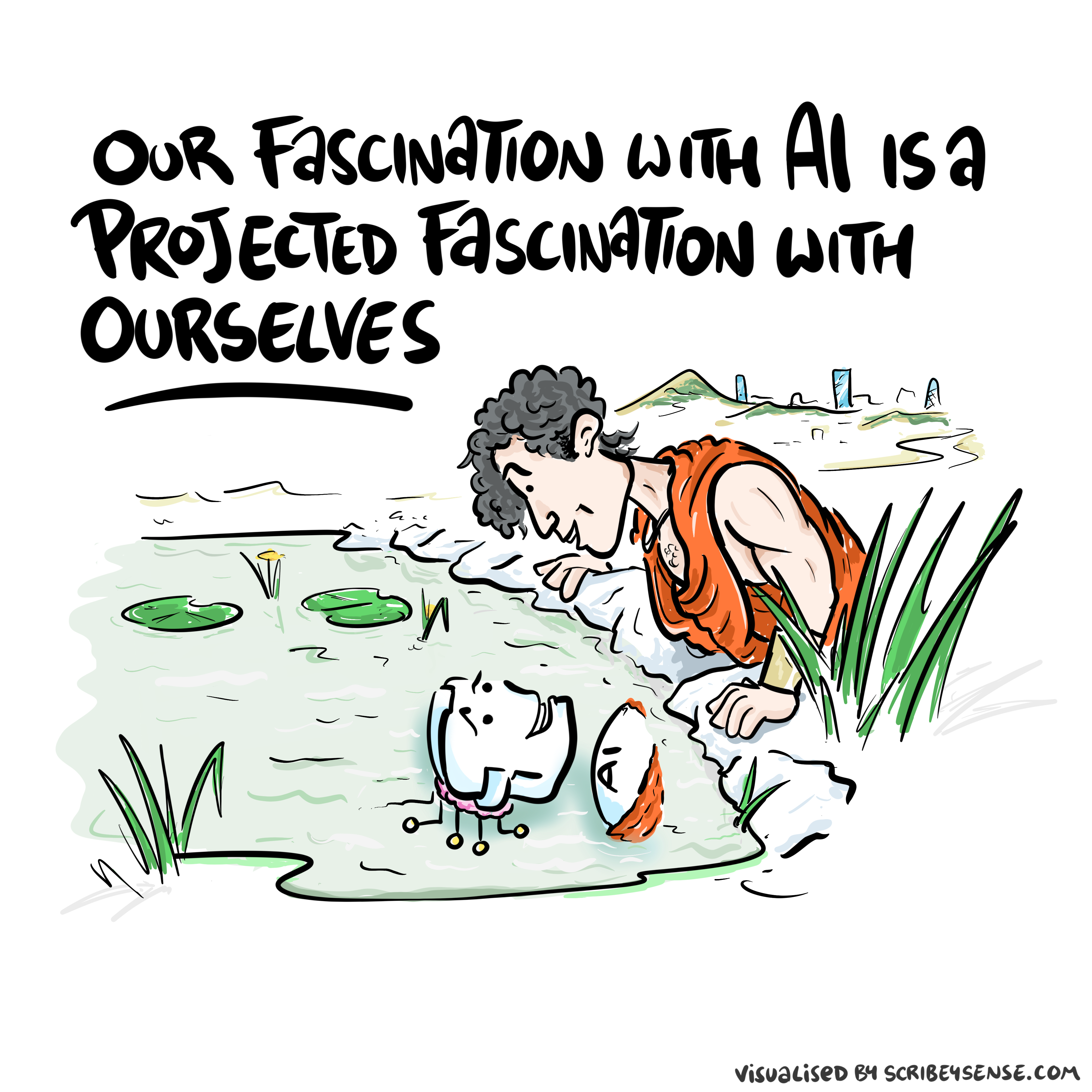
Figure: This is the drawing Dan was inspired to create for Chapter 1. It captures the fundamentally narcissistic nature of our (societal) obsession with our intelligence.

See blog post on Dan Andrews image of our reflective obsession with AI.. See also (Vallor, 2024).

Part 2: How AI Changes the Firm

[edit]

The Attention Economy

[edit]

Human intelligence is locked-in. It’s bandwidth restricted. This makes it a bottleneck in the attention economy.

Herbert Simon on Information

[edit]

What information consumes is rather obvious: it consumes the attention of its recipients. Hence a wealth of information creates a poverty of attention …
Simon (1971)

The attention economy was a phenomenon described in 1971 by the American computer scientist Herbert Simon. He saw the coming information revolution and wrote that a wealth of information would create a poverty of attention. Too much information means that human attention becomes the scarce resource, the bottleneck. It becomes the gold in the attention economy.

The power associated with control of information dates back to the invention of writing. By pressing reeds into clay tablets Sumerian scribes stored information and controlled the flow of information.

New Flow of Information

[edit]

Classically the field of statistics focused on mediating the relationship between the machine and the human. Our limited bandwidth of communication means we tend to over-interpret the limited information that we are given, in the extreme we assign motives and desires to inanimate objects (a process known as anthropomorphizing). Much of mathematical statistics was developed to help temper this tendency and understand when we are valid in drawing conclusions from data.

Figure: The trinity of human, data, and computer, and highlights the modern phenomenon. The communication channel between computer and data now has an extremely high bandwidth. The channel between human and computer and the channel between data and human is narrow. New direction of information flow, information is reaching us mediated by the computer. The focus on classical statistics reflected the importance of the direct communication between human and data. The modern challenges of data science emerge when that relationship is being mediated by the machine.

Data science brings new challenges. In particular, there is a very large bandwidth connection between the machine and data. This means that our relationship with data is now commonly being mediated by the machine. Whether this is in the acquisition of new data, which now happens by happenstance rather than with purpose, or the interpretation of that data where we are increasingly relying on machines to summarize what the data contains. This is leading to the emerging field of data science, which must not only deal with the same challenges that mathematical statistics faced in tempering our tendency to over interpret data but must also deal with the possibility that the machine has either inadvertently or maliciously misrepresented the underlying data.

See Lawrence (2024) topography, information p. 34-9, 43-8, 57, 62, 104, 115-16, 127, 140, 192, 196, 199, 291, 334, 354-5. See Lawrence (2024) anthropomorphization (‘anthrox’) p. 30-31, 90-91, 93-4, 100, 132, 148, 153, 163, 216-17, 239, 276, 326, 342.

Institutional Character

[edit]

Before we start, I’d like to highlight one idea that will be key for contextualisation of everything else. There is a strong interaction between the structure of an organisation and the structure of its software.

This is known as Conway’s law:

Organizations, who design systems, are constrained to produce designs which are copies of the communication structures of these organizations.
Melvin Conway Conway (n.d.)

The API Mandate

[edit]

The API Mandate was a memo issued by Jeff Bezos in 2002. Internet folklore has the memo making five statements:

All teams will henceforth expose their data and functionality through service interfaces.
Teams must communicate with each other through these interfaces.
There will be no other form of inter-process communication allowed: no direct linking, no direct reads of another team’s data store, no shared-memory model, no back-doors whatsoever. The only communication allowed is via service interface calls over the network.
It doesn’t matter what technology they use.
All service interfaces, without exception, must be designed from the ground up to be externalizable. That is to say, the team must plan and design to be able to expose the interface to developers in the outside world. No exceptions.

The mandate marked a shift in the way Amazon viewed software, moving to a model that dominates the way software is built today, so-called “Software-as-a-Service.”

Any organization that designs a system (defined broadly) will produce a design whose structure is a copy of the organization’s communication structure.
Conway (n.d.)

The law is cited in the classic software engineering text, The Mythical Man Month (Brooks, n.d.).

As a result, and in awareness of Conway’s law, the implementation of this mandate also had a dramatic effect on Amazon’s organizational structure.

Because the design that occurs first is almost never the best possible, the prevailing system concept may need to change. Therefore, flexibility of organization is important to effective design.
Conway (n.d.)

Amazon is set up around the notion of the “two pizza team.” Teams of 6-10 people that can be theoretically fed by two (American) pizzas. This structure is tightly interconnected with the software. Each of these teams owns one of these “services.” Amazon is strict about the team that develops the service owning the service in production. This approach is the secret to their scale as a company, and the approach has been adopted by many other large tech companies. The software-as-a-service approach changed the information infrastructure of the company. The routes through which information is shared. This had a knock-on effect on the corporate culture.

Amazon works through an approach I think of as “devolved autonomy.” The culture of the company is widely taught (e.g. Customer Obsession, Ownership, Frugality), a team’s inputs and outputs are strictly defined, but within those parameters, teams have a great of autonomy in how they operate. The information infrastructure was devolved, so the autonomy was devolved. The different parts of Amazon are then bound together through shared corporate culture.

Amazon prides itself on agility, I spent three years there and I can confirm things move very quickly. I used to joke that just as a dog year is seven normal years, an Amazon year is four normal years in any other company.

Not all institutions move quickly. My current role is at the University of Cambridge. There are similarities between the way a University operates and the way Amazon operates. In particular Universities exploit devolved autonomy to empower their research leads.

Naturally there are differences too, for example, Universities do less work on developing culture. Corporate culture is a critical element in ensuring that despite the devolved autonomy of Amazon, there is a common vision.

Cambridge University is over 800 years old. Agility is not a word that is commonly used to describe its institutional framework. I don’t want to make a claim for whether an agile institution is better or worse, it’s circumstantial. Institutions have characters, like people. The institutional character of the University is the one of a steady and reliable friend. The institutional character of Amazon is more mecurial.

Why do I emphasise this? Because when it comes to organisational data science, when it comes to a data driven culture around our decision making, that culture inter-plays with the institutional character. If decision making is truly data-driven, then we should expect co-evolution between the information infrastructure and the institutional structures.

A common mistake I’ve seen is to transplant a data culture from one (ostensibly) successful institution to another. Such transplants commonly lead to organisational rejection. The institutional character of the new host will have cultural antibodies that operate against the transplant even if, at some (typically executive) level the institution is aware of the vital need for integrating the data driven culture.

A major part of my job at Amazon was dealing with these tensions. As a scientist, initially working across the company, working with my team introduced dependencies and practices that impinged on the devolved autonomy. I face a similar challenge at Cambridge. Our aim is to integrate data driven methodologies with the classical sciences, humanities and across the academic spectrum. The devolved autonomy inherent in University research provides a similar set of challenges to those I faced at Amazon.

My role before Amazon was at the University of Sheffield. Those were quieter times in terms of societal interest in machine learning and data science, but the Royal Society was already convening a working group on Machine Learning. This was my first interaction with policy advice, I’ve continued that interaction today by working with the AI Council, convening the DELVE group to give pandemic advice, serving on the Advisory Council for the Centre for Science and Policy, and the Advisory Board for the Centre for Data Ethics and Innovation. I’m not an expert on the civil service and government, but I believe many of the themes I’ve outlined above also apply within government. The ideas I’ll talk about today build on the experiences I’ve had at Sheffield, Amazon, and Cambridge alongside the policy work I’ve been involved in to make suggestions of what the barriers are for enabling a culture of data driven policy making.

The Horizon scandal

[edit]

In the UK we saw these effects play out in the Horizon scandal: the accounting system of the national postal service was computerized by Fujitsu and first installed in 1999, but neither the Post Office nor Fujitsu were able to control the system they had deployed. When it went wrong individual sub postmasters were blamed for the systems’ errors. Over the next two decades they were prosecuted and jailed leaving lives ruined in the wake of the machine’s mistakes.

Figure: The still is from the 2015 select committee.

See Lawrence (2024) Horizon scandal p. 371.

Part 3: Competing Globally with AI

Productivity Flywheel

[edit]

Figure: The productivity flywheel suggests technical innovation is reinvested.

The productivity flywheel should return the gains released by productivity through funding. This relies on the economic value mapping the underlying value.

Supply Chain of Ideas

[edit]

Model is “supply chain of ideas” framework, particularly in the context of information technology and AI solutions like machine learning and large language models. You suggest that this idea flow, from creation to application, is similar to how physical goods move through economic supply chains.

In the realm of IT solutions, there’s been an overemphasis on macro-economic “supply-side” stimulation - focusing on creating new technologies and ideas - without enough attention to the micro-economic “demand-side” - understanding and addressing real-world needs and challenges.

Imagining the supply chain rather than just the notion of the Innovation Economy allows the conceptualisation of the gaps between macro and micro economic issues, enabling a different way of thinking about process innovation.

Phrasing things in terms of a supply chain of ideas suggests that innovation requires both characterisation of the demand and the supply of ideas. This leads to four key elements:

Multiple sources of ideas (diversity)
Efficient delivery mechanisms
Quick deployment capabilities
Customer-driven prioritization

The next priority is mapping the demand for ideas to the supply of ideas. This is where much of our innovation system is failing. In supply chain optimisaiton a large effort is spent on understanding current stock and managing resources to bring the supply to map to the demand. This includes shaping the supply as well as managing it.

The objective is to create a system that can generate, evaluate, and deploy ideas efficiently and effectively, while ensuring that people’s needs and preferences are met. The customer here depends on the context - it could be the public, it could be a business, it could be a government department but very often it’s individual citizens. The loss of their voice in the innovation economy is a trigger for the gap between the innovation supply (at a macro level) and the innovation demand (at a micro level).

For students of international competition: AI does not erase geography, regulation, or culture. It changes the speed and shape of information inside the firm, and therefore where advantage and failure modes appear when companies operate across borders.

Thanks!

For more information on these subjects and more you might want to check the following resources.

References

Brooks, F., n.d. The mythical man-month. Addison-Wesley.

Conway, M.E., n.d. How do committees invent? Datamation 14, 28–31.

Lawrence, N.D., 2024. The atomic human: Understanding ourselves in the age of AI. Allen Lane.

Simon, H.A., 1971. Designing organizations for an information-rich world. Johns Hopkins University Press, Baltimore, MD.

Vallor, S., 2024. The AI mirror. Oxford University Press.