AI Can’t Fix This: Happenstance Data, Modelling, and the Covid19 Pandemic

Neil D. Lawrence

$$\newcommand{\tk}[1]{} \newcommand{\Amatrix}{\mathbf{A}} \newcommand{\KL}[2]{\text{KL}\left( #1\,\|\,#2 \right)} \newcommand{\Kaast}{\kernelMatrix_{\mathbf{ \ast}\mathbf{ \ast}}} \newcommand{\Kastu}{\kernelMatrix_{\mathbf{ \ast} \inducingVector}} \newcommand{\Kff}{\kernelMatrix_{\mappingFunctionVector \mappingFunctionVector}} \newcommand{\Kfu}{\kernelMatrix_{\mappingFunctionVector \inducingVector}} \newcommand{\Kuast}{\kernelMatrix_{\inducingVector \bf\ast}} \newcommand{\Kuf}{\kernelMatrix_{\inducingVector \mappingFunctionVector}} \newcommand{\Kuu}{\kernelMatrix_{\inducingVector \inducingVector}} \newcommand{\Kuui}{\Kuu^{-1}} \newcommand{\Qaast}{\mathbf{Q}_{\bf \ast \ast}} \newcommand{\Qastf}{\mathbf{Q}_{\ast \mappingFunction}} \newcommand{\Qfast}{\mathbf{Q}_{\mappingFunctionVector \bf \ast}} \newcommand{\Qff}{\mathbf{Q}_{\mappingFunctionVector \mappingFunctionVector}} \newcommand{\aMatrix}{\mathbf{A}} \newcommand{\aScalar}{a} \newcommand{\aVector}{\mathbf{a}} \newcommand{\acceleration}{a} \newcommand{\bMatrix}{\mathbf{B}} \newcommand{\bScalar}{b} \newcommand{\bVector}{\mathbf{b}} \newcommand{\basisFunc}{\phi} \newcommand{\basisFuncVector}{\boldsymbol{ \basisFunc}} \newcommand{\basisFunction}{\phi} \newcommand{\basisLocation}{\mu} \newcommand{\basisMatrix}{\boldsymbol{ \Phi}} \newcommand{\basisScalar}{\basisFunction} \newcommand{\basisVector}{\boldsymbol{ \basisFunction}} \newcommand{\activationFunction}{\phi} \newcommand{\activationMatrix}{\boldsymbol{ \Phi}} \newcommand{\activationScalar}{\basisFunction} \newcommand{\activationVector}{\boldsymbol{ \basisFunction}} \newcommand{\bigO}{\mathcal{O}} \newcommand{\binomProb}{\pi} \newcommand{\cMatrix}{\mathbf{C}} \newcommand{\cbasisMatrix}{\hat{\boldsymbol{ \Phi}}} \newcommand{\cdataMatrix}{\hat{\dataMatrix}} \newcommand{\cdataScalar}{\hat{\dataScalar}} \newcommand{\cdataVector}{\hat{\dataVector}} \newcommand{\centeredKernelMatrix}{\mathbf{ \MakeUppercase{\centeredKernelScalar}}} \newcommand{\centeredKernelScalar}{b} \newcommand{\centeredKernelVector}{\centeredKernelScalar} \newcommand{\centeringMatrix}{\mathbf{H}} \newcommand{\chiSquaredDist}[2]{\chi_{#1}^{2}\left(#2\right)} \newcommand{\chiSquaredSamp}[1]{\chi_{#1}^{2}} \newcommand{\conditionalCovariance}{\boldsymbol{ \Sigma}} \newcommand{\coregionalizationMatrix}{\mathbf{B}} \newcommand{\coregionalizationScalar}{b} \newcommand{\coregionalizationVector}{\mathbf{ \coregionalizationScalar}} \newcommand{\covDist}[2]{\text{cov}_{#2}\left(#1\right)} \newcommand{\covSamp}[1]{\text{cov}\left(#1\right)} \newcommand{\covarianceScalar}{c} \newcommand{\covarianceVector}{\mathbf{ \covarianceScalar}} \newcommand{\covarianceMatrix}{\mathbf{C}} \newcommand{\covarianceMatrixTwo}{\boldsymbol{ \Sigma}} \newcommand{\croupierScalar}{s} \newcommand{\croupierVector}{\mathbf{ \croupierScalar}} \newcommand{\croupierMatrix}{\mathbf{ \MakeUppercase{\croupierScalar}}} \newcommand{\dataDim}{p} \newcommand{\dataIndex}{i} \newcommand{\dataIndexTwo}{j} \newcommand{\dataMatrix}{\mathbf{Y}} \newcommand{\dataScalar}{y} \newcommand{\dataSet}{\mathcal{D}} \newcommand{\dataStd}{\sigma} \newcommand{\dataVector}{\mathbf{ \dataScalar}} \newcommand{\decayRate}{d} \newcommand{\degreeMatrix}{\mathbf{ \MakeUppercase{\degreeScalar}}} \newcommand{\degreeScalar}{d} \newcommand{\degreeVector}{\mathbf{ \degreeScalar}} \newcommand{\diag}[1]{\text{diag}\left(#1\right)} \newcommand{\diagonalMatrix}{\mathbf{D}} \newcommand{\diff}[2]{\frac{\text{d}#1}{\text{d}#2}} \newcommand{\diffTwo}[2]{\frac{\text{d}^2#1}{\text{d}#2^2}} \newcommand{\displacement}{x} \newcommand{\displacementVector}{\textbf{\displacement}} \newcommand{\distanceMatrix}{\mathbf{ \MakeUppercase{\distanceScalar}}} \newcommand{\distanceScalar}{d} \newcommand{\distanceVector}{\mathbf{ \distanceScalar}} \newcommand{\eigenvaltwo}{\ell} \newcommand{\eigenvaltwoMatrix}{\mathbf{L}} \newcommand{\eigenvaltwoVector}{\mathbf{l}} \newcommand{\eigenvalue}{\lambda} \newcommand{\eigenvalueMatrix}{\boldsymbol{ \Lambda}} \newcommand{\eigenvalueVector}{\boldsymbol{ \lambda}} \newcommand{\eigenvector}{\mathbf{ \eigenvectorScalar}} \newcommand{\eigenvectorMatrix}{\mathbf{U}} \newcommand{\eigenvectorScalar}{u} \newcommand{\eigenvectwo}{\mathbf{v}} \newcommand{\eigenvectwoMatrix}{\mathbf{V}} \newcommand{\eigenvectwoScalar}{v} \newcommand{\entropy}[1]{\mathcal{H}\left(#1\right)} \newcommand{\errorFunction}{E} \newcommand{\expDist}[2]{\left\langle#1\right\rangle_{#2}} \newcommand{\expSamp}[1]{\left\langle#1\right\rangle} \newcommand{\expectation}[1]{\left\langle #1 \right\rangle } \newcommand{\expectationDist}[2]{\left\langle #1 \right\rangle _{#2}} \newcommand{\expectedDistanceMatrix}{\mathcal{D}} \newcommand{\eye}{\mathbf{I}} \newcommand{\fantasyDim}{r} \newcommand{\fantasyMatrix}{\mathbf{ \MakeUppercase{\fantasyScalar}}} \newcommand{\fantasyScalar}{z} \newcommand{\fantasyVector}{\mathbf{ \fantasyScalar}} \newcommand{\featureStd}{\varsigma} \newcommand{\gammaCdf}[3]{\mathcal{GAMMA CDF}\left(#1|#2,#3\right)} \newcommand{\gammaDist}[3]{\mathcal{G}\left(#1|#2,#3\right)} \newcommand{\gammaSamp}[2]{\mathcal{G}\left(#1,#2\right)} \newcommand{\gaussianDist}[3]{\mathcal{N}\left(#1|#2,#3\right)} \newcommand{\gaussianSamp}[2]{\mathcal{N}\left(#1,#2\right)} \newcommand{\uniformDist}[3]{\mathcal{U}\left(#1|#2,#3\right)} \newcommand{\uniformSamp}[2]{\mathcal{U}\left(#1,#2\right)} \newcommand{\given}{|} \newcommand{\half}{\frac{1}{2}} \newcommand{\heaviside}{H} \newcommand{\hiddenMatrix}{\mathbf{ \MakeUppercase{\hiddenScalar}}} \newcommand{\hiddenScalar}{h} \newcommand{\hiddenVector}{\mathbf{ \hiddenScalar}} \newcommand{\identityMatrix}{\eye} \newcommand{\inducingInputScalar}{z} \newcommand{\inducingInputVector}{\mathbf{ \inducingInputScalar}} \newcommand{\inducingInputMatrix}{\mathbf{Z}} \newcommand{\inducingScalar}{u} \newcommand{\inducingVector}{\mathbf{ \inducingScalar}} \newcommand{\inducingMatrix}{\mathbf{U}} \newcommand{\inlineDiff}[2]{\text{d}#1/\text{d}#2} \newcommand{\inputDim}{q} \newcommand{\inputMatrix}{\mathbf{X}} \newcommand{\inputScalar}{x} \newcommand{\inputSpace}{\mathcal{X}} \newcommand{\inputVals}{\inputVector} \newcommand{\inputVector}{\mathbf{ \inputScalar}} \newcommand{\iterNum}{k} \newcommand{\kernel}{\kernelScalar} \newcommand{\kernelMatrix}{\mathbf{K}} \newcommand{\kernelScalar}{k} \newcommand{\kernelVector}{\mathbf{ \kernelScalar}} \newcommand{\kff}{\kernelScalar_{\mappingFunction \mappingFunction}} \newcommand{\kfu}{\kernelVector_{\mappingFunction \inducingScalar}} \newcommand{\kuf}{\kernelVector_{\inducingScalar \mappingFunction}} \newcommand{\kuu}{\kernelVector_{\inducingScalar \inducingScalar}} \newcommand{\lagrangeMultiplier}{\lambda} \newcommand{\lagrangeMultiplierMatrix}{\boldsymbol{ \Lambda}} \newcommand{\lagrangian}{L} \newcommand{\laplacianFactor}{\mathbf{ \MakeUppercase{\laplacianFactorScalar}}} \newcommand{\laplacianFactorScalar}{m} \newcommand{\laplacianFactorVector}{\mathbf{ \laplacianFactorScalar}} \newcommand{\laplacianMatrix}{\mathbf{L}} \newcommand{\laplacianScalar}{\ell} \newcommand{\laplacianVector}{\mathbf{ \ell}} \newcommand{\latentDim}{q} \newcommand{\latentDistanceMatrix}{\boldsymbol{ \Delta}} \newcommand{\latentDistanceScalar}{\delta} \newcommand{\latentDistanceVector}{\boldsymbol{ \delta}} \newcommand{\latentForce}{f} \newcommand{\latentFunction}{u} \newcommand{\latentFunctionVector}{\mathbf{ \latentFunction}} \newcommand{\latentFunctionMatrix}{\mathbf{ \MakeUppercase{\latentFunction}}} \newcommand{\latentIndex}{j} \newcommand{\latentScalar}{z} \newcommand{\latentVector}{\mathbf{ \latentScalar}} \newcommand{\latentMatrix}{\mathbf{Z}} \newcommand{\learnRate}{\eta} \newcommand{\lengthScale}{\ell} \newcommand{\rbfWidth}{\ell} \newcommand{\likelihoodBound}{\mathcal{L}} \newcommand{\likelihoodFunction}{L} \newcommand{\locationScalar}{\mu} \newcommand{\locationVector}{\boldsymbol{ \locationScalar}} \newcommand{\locationMatrix}{\mathbf{M}} \newcommand{\variance}[1]{\text{var}\left( #1 \right)} \newcommand{\mappingFunction}{f} \newcommand{\mappingFunctionMatrix}{\mathbf{F}} \newcommand{\mappingFunctionTwo}{g} \newcommand{\mappingFunctionTwoMatrix}{\mathbf{G}} \newcommand{\mappingFunctionTwoVector}{\mathbf{ \mappingFunctionTwo}} \newcommand{\mappingFunctionVector}{\mathbf{ \mappingFunction}} \newcommand{\scaleScalar}{s} \newcommand{\mappingScalar}{w} \newcommand{\mappingVector}{\mathbf{ \mappingScalar}} \newcommand{\mappingMatrix}{\mathbf{W}} \newcommand{\mappingScalarTwo}{v} \newcommand{\mappingVectorTwo}{\mathbf{ \mappingScalarTwo}} \newcommand{\mappingMatrixTwo}{\mathbf{V}} \newcommand{\maxIters}{K} \newcommand{\meanMatrix}{\mathbf{M}} \newcommand{\meanScalar}{\mu} \newcommand{\meanTwoMatrix}{\mathbf{M}} \newcommand{\meanTwoScalar}{m} \newcommand{\meanTwoVector}{\mathbf{ \meanTwoScalar}} \newcommand{\meanVector}{\boldsymbol{ \meanScalar}} \newcommand{\mrnaConcentration}{m} \newcommand{\naturalFrequency}{\omega} \newcommand{\neighborhood}[1]{\mathcal{N}\left( #1 \right)} \newcommand{\neilurl}{http://inverseprobability.com/} \newcommand{\noiseMatrix}{\boldsymbol{ E}} \newcommand{\noiseScalar}{\epsilon} \newcommand{\noiseVector}{\boldsymbol{ \epsilon}} \newcommand{\noiseStd}{\sigma} \newcommand{\norm}[1]{\left\Vert #1 \right\Vert} \newcommand{\normalizedLaplacianMatrix}{\hat{\mathbf{L}}} \newcommand{\normalizedLaplacianScalar}{\hat{\ell}} \newcommand{\normalizedLaplacianVector}{\hat{\mathbf{ \ell}}} \newcommand{\numActive}{m} \newcommand{\numBasisFunc}{m} \newcommand{\numComponents}{m} \newcommand{\numComps}{K} \newcommand{\numData}{n} \newcommand{\numFeatures}{K} \newcommand{\numHidden}{h} \newcommand{\numInducing}{m} \newcommand{\numLayers}{\ell} \newcommand{\numNeighbors}{K} \newcommand{\numSequences}{s} \newcommand{\numSuccess}{s} \newcommand{\numTasks}{m} \newcommand{\numTime}{T} \newcommand{\numTrials}{S} \newcommand{\outputIndex}{j} \newcommand{\paramVector}{\boldsymbol{ \theta}} \newcommand{\parameterMatrix}{\boldsymbol{ \Theta}} \newcommand{\parameterScalar}{\theta} \newcommand{\parameterVector}{\boldsymbol{ \parameterScalar}} \newcommand{\partDiff}[2]{\frac{\partial#1}{\partial#2}} \newcommand{\precisionScalar}{j} \newcommand{\precisionVector}{\mathbf{ \precisionScalar}} \newcommand{\precisionMatrix}{\mathbf{J}} \newcommand{\pseudotargetScalar}{\widetilde{y}} \newcommand{\pseudotargetVector}{\mathbf{ \pseudotargetScalar}} \newcommand{\pseudotargetMatrix}{\mathbf{ \widetilde{Y}}} \newcommand{\rank}[1]{\text{rank}\left(#1\right)} \newcommand{\rayleighDist}[2]{\mathcal{R}\left(#1|#2\right)} \newcommand{\rayleighSamp}[1]{\mathcal{R}\left(#1\right)} \newcommand{\responsibility}{r} \newcommand{\rotationScalar}{r} \newcommand{\rotationVector}{\mathbf{ \rotationScalar}} \newcommand{\rotationMatrix}{\mathbf{R}} \newcommand{\sampleCovScalar}{s} \newcommand{\sampleCovVector}{\mathbf{ \sampleCovScalar}} \newcommand{\sampleCovMatrix}{\mathbf{s}} \newcommand{\scalarProduct}[2]{\left\langle{#1},{#2}\right\rangle} \newcommand{\sign}[1]{\text{sign}\left(#1\right)} \newcommand{\sigmoid}[1]{\sigma\left(#1\right)} \newcommand{\singularvalue}{\ell} \newcommand{\singularvalueMatrix}{\mathbf{L}} \newcommand{\singularvalueVector}{\mathbf{l}} \newcommand{\sorth}{\mathbf{u}} \newcommand{\spar}{\lambda} \newcommand{\trace}[1]{\text{tr}\left(#1\right)} \newcommand{\BasalRate}{B} \newcommand{\DampingCoefficient}{C} \newcommand{\DecayRate}{D} \newcommand{\Displacement}{X} \newcommand{\LatentForce}{F} \newcommand{\Mass}{M} \newcommand{\Sensitivity}{S} \newcommand{\basalRate}{b} \newcommand{\dampingCoefficient}{c} \newcommand{\mass}{m} \newcommand{\sensitivity}{s} \newcommand{\springScalar}{\kappa} \newcommand{\springVector}{\boldsymbol{ \kappa}} \newcommand{\springMatrix}{\boldsymbol{ \mathcal{K}}} \newcommand{\tfConcentration}{p} \newcommand{\tfDecayRate}{\delta} \newcommand{\tfMrnaConcentration}{f} \newcommand{\tfVector}{\mathbf{ \tfConcentration}} \newcommand{\velocity}{v} \newcommand{\sufficientStatsScalar}{g} \newcommand{\sufficientStatsVector}{\mathbf{ \sufficientStatsScalar}} \newcommand{\sufficientStatsMatrix}{\mathbf{G}} \newcommand{\switchScalar}{s} \newcommand{\switchVector}{\mathbf{ \switchScalar}} \newcommand{\switchMatrix}{\mathbf{S}} \newcommand{\tr}[1]{\text{tr}\left(#1\right)} \newcommand{\loneNorm}[1]{\left\Vert #1 \right\Vert_1} \newcommand{\ltwoNorm}[1]{\left\Vert #1 \right\Vert_2} \newcommand{\onenorm}[1]{\left\vert#1\right\vert_1} \newcommand{\twonorm}[1]{\left\Vert #1 \right\Vert} \newcommand{\vScalar}{v} \newcommand{\vVector}{\mathbf{v}} \newcommand{\vMatrix}{\mathbf{V}} \newcommand{\varianceDist}[2]{\text{var}_{#2}\left( #1 \right)} \newcommand{\vecb}[1]{\left(#1\right):} \newcommand{\weightScalar}{w} \newcommand{\weightVector}{\mathbf{ \weightScalar}} \newcommand{\weightMatrix}{\mathbf{W}} \newcommand{\weightedAdjacencyMatrix}{\mathbf{A}} \newcommand{\weightedAdjacencyScalar}{a} \newcommand{\weightedAdjacencyVector}{\mathbf{ \weightedAdjacencyScalar}} \newcommand{\onesVector}{\mathbf{1}} \newcommand{\zerosVector}{\mathbf{0}} $$

at The Flip Side of the Pandemic: Recent Advances in the Mathematics of Information on May 20, 2021 [reveal]

Neil D. Lawrence, University of Cambridge

Abstract

With the world watching case numbers increase and publics and policymakers scrutinising projections from epidemiological models, the covid-19 pandemic brought with it increased attention on the use of data to inform policy. Alongside this scrutiny came a new wave of interest in the ability of data and artificial intelligence (AI) to help tackle major scientific and social challenges: could our increasing ability to collect, combine and interrogate large datasets lead to new insights that unlock more effective policy responses? Experiences from the DELVE Initiative, convened to bring data science to bear on covid-19 policy, suggests achieving this aim requires wider adoption of open data science methods to deploy data science and AI expertise and resources to tackle real-world problems.

Lies and Damned Lies

[edit]

There are three types of lies: lies, damned lies and statistics

Benjamin Disraeli 1804-1881

Benjamin Disraeli said¹ that there three types of lies: lies, damned lies and statistics. Disraeli died in 1881, 30 years before the first academic department of applied statistics was founded at UCL. If Disraeli were alive today, it is likely that he’d rephrase his quote:

There are three types of lies, lies damned lies and big data.

Why? Because the challenges of understanding and interpreting big data today are similar to those that Disraeli faced in governing an empire through statistics in the latter part of the 19th century.

The quote lies, damned lies and statistics was credited to Benjamin Disraeli by Mark Twain in his autobiography. It characterizes the idea that statistic can be made to prove anything. But Disraeli died in 1881 and Mark Twain died in 1910. The important breakthrough in overcoming our tendency to overinterpet data came with the formalization of the field through the development of mathematical statistics.

Data has an elusive quality, it promises so much but can deliver little, it can mislead and misrepresent. To harness it, it must be tamed. In Disraeli’s time during the second half of the 19th century, numbers and data were being accumulated, the social sciences were being developed. There was a large scale collection of data for the purposes of government.

The modern ‘big data era’ is on the verge of delivering the same sense of frustration that Disraeli experienced, the early promise of big data as a panacea is evolving to demands for delivery. For me, personally, peak-hype coincided with an email I received inviting collaboration on a project to deploy “Big Data and Internet of Things in an Industry 4.0 environment.” Further questioning revealed that the actual project was optimization of the efficiency of a manufacturing production line, a far more tangible and realizable goal.

The antidote to this verbage is found in increasing awareness. When dealing with data the first trap to avoid is the games of buzzword bingo that we are wont to play. The first goal is to quantify what challenges can be addressed and what techniques are required. Behind the hype fundamentals are changing. The phenomenon is about the increasing access we have to data. The manner in which customers information is recorded and processes are codified and digitized with little overhead. Internet of things is about the increasing number of cheap sensors that can be easily interconnected through our modern network structures. But businesses are about making money, and these phenomena need to be recast in those terms before their value can be realized.

Mathematical Statistics

Karl Pearson (1857-1936), Ronald Fisher (1890-1962) and others considered the question of what conclusions can truly be drawn from data. Their mathematical studies act as a restraint on our tendency to over-interpret and see patterns where there are none. They introduced concepts such as randomized control trials that form a mainstay of the our decision making today, from government, to clinicians to large scale A/B testing that determines the nature of the web interfaces we interact with on social media and shopping.

Figure: Karl Pearson (1857-1936), one of the founders of Mathematical Statistics.

Their movement did the most to put statistics to rights, to eradicate the ‘damned lies.’ It was known as ‘mathematical statistics’. Today I believe we should look to the emerging field of data science to provide the same role. Data science is an amalgam of statistics, data mining, computer systems, databases, computation, machine learning and artificial intelligence. Spread across these fields are the tools we need to realize data’s potential. For many businesses this might be thought of as the challenge of ‘converting bits into atoms.’ Bits: the data stored on computer, atoms: the physical manifestation of what we do; the transfer of goods, the delivery of service. From fungible to tangible. When solving a challenge through data there are a series of obstacles that need to be addressed.

Firstly, data awareness: what data you have and where its stored. Sometimes this includes changing your conception of what data is and how it can be obtained. From automated production lines to apps on employee smart phones. Often data is locked away: manual log books, confidential data, personal data. For increasing awareness an internal audit can help. The website data.gov.uk hosts data made available by the UK government. To create this website the government’s departments went through an audit of what data they each hold and what data they could make available. Similarly, within private buisnesses this type of audit could be useful for understanding their internal digital landscape: after all the key to any successful campaign is a good map.

Secondly, availability. How well are the data sources interconnected? How well curated are they? The curse of Disraeli was associated with unreliable data and unreliable statistics. The misrepresentations this leads to are worse than the absence of data as they give a false sense of confidence to decision making. Understanding how to avoid these pitfalls involves an improved sense of data and its value, one that needs to permeate the organization.

The final challenge is analysis, the accumulation of the necessary expertise to digest what the data tells us. Data requires intepretation, and interpretation requires experience. Analysis is providing a bottleneck due to a skill shortage, a skill shortage made more acute by the fact that, ideally, analysis should be carried out by individuals not only skilled in data science but also equipped with the domain knowledge to understand the implications in a given application, and to see opportunities for improvements in efficiency.

‘Mathematical Data Science’

As a term ‘big data’ promises much and delivers little, to get true value from data, it needs to be curated and evaluated. The three stages of awareness, availability and analysis provide a broad framework through which organizations should be assessing the potential in the data they hold. Hand waving about big data solutions will not do, it will only lead to self-deception. The castles we build on our data landscapes must be based on firm foundations, process and scientific analysis. If we do things right, those are the foundations that will be provided by the new field of data science.

Today the statement “There are three types of lies: lies, damned lies and ‘big data’” may be more apt. We are revisiting many of the mistakes made in interpreting data from the 19th century. Big data is laid down by happenstance, rather than actively collected with a particular question in mind. That means it needs to be treated with care when conclusions are being drawn. For data science to succede it needs the same form of rigour that Pearson and Fisher brought to statistics, a “mathematical data science” is needed.

You can also check my blog post on Lies, Damned Lies and Big Data.

DELVE Overview

[edit]

The DELVE Initiative was convened by the Royal Society early in the pandemic in response for a perceived need to increase provide policy advice for the UK’s response to covide, with an initial focus on exit strategy from the first lock down.

Figure: The Royal Society announces the DELVE group to tackle the COVID-19 crisis. https://royalsociety.org/news/2020/04/royal-society-convenes-data-analytics-group-to-tackle-COVID-19/.

DELVE will contribute data driven analysis to complement the evidence base informing the UK’s strategic response, by:

Analysing national and international data to determine the effect of different measures and strategies on a range of public health, social and economic outcomes

Using emerging sources of data as new evidence from the unfolding pandemic comes to light

Ensuring that the work of this group is coordinated with others and communicated as necessary both nationally and internationally

Delve Timeline

[edit]

First contact 3rd April
First meeting 7th April
First working group 16th April

The Delve initiative is a group that was convened by the Royal Society to help provide data-driven insights about the pandemic, with an initial focus on exiting the first lockdown and particular interest in using the variation of strategies across different international governments to inform policy.

Right from the start, data was at the heart of what DELVE does, but the reality is that little can be done without domain expertise and often the data we required wasn’t available.

However, even when it is not present, the notion of what data might be needed can also have a convening effect, bringing together multiple disciplines around the policy questons at hand. The Delve Data Readiness report (The DELVE Initiative, 2020a) makes recommendations for how we can improve our processes around data, but this talk also focuses on how data brings different disciplines together around data.

Any policy question can be framed in a number of different ways - what are the health outcomes; what is the impact on NHS capacity; how are different groups affected; what is the economic impact – and each has different types of evidence associated with it. Complex and uncertain challenges require efforts to draw insights together from across disciplines.

Sustained engagement between government and academia plays an important role in building mutual understanding about what each can deliver. Core to DELVE’s work was the intention that research questions be framed in ways that would resonate with the policy challenges being seen in government.

What is Machine Learning?

\[ \text{data} + \text{model} \stackrel{\text{compute}}{\rightarrow} \text{prediction}\]

The Big Data Paradox

[edit]

The big data paradox is the modern phenomenon of “as we collect more data, we understand less.” It is emerging in several domains, political polling, characterization of patients for trials data, monitoring twitter for political sentiment.

I like to think of the phenomenon as relating to the notion of “can’t see the wood for the trees.” Classical statistics, with randomized controlled trials, improved society’s understanding of data. It improved our ability to monitor the forest, to consider population health, voting patterns etc. It is critically dependent on active approaches to data collection that deal with confounders. This data collection can be very expensive.

In business today, it is still the gold standard, A/B tests are used to understand the effect of an intervention on revenue or customer capture or supply chain costs.

Figure: New beech leaves growing in the Gribskov Forest in the northern part of Sealand, Denmark. Photo from wikimedia commons by Malene Thyssen, http://commons.wikimedia.org/wiki/User:Malene.

The new phenomenon is happenstance data. Data that is not actively collected with a question in mind. As a result, it can mislead us. For example, if we assume the politics of active users of twitter is reflective of the wider population’s politics, then we may be misled.

However, this happenstance data often allows us to characterise a particular individual to a high degree of accuracy. Classical statistics was all about the forest, but big data can often become about the individual tree. As a result we are misled about the situation.

The phenomenon is more dangerous, because our perception is that we are characterizing the wider scenario with ever increasing accuracy. Whereas we are just becoming distracted by detail that may or may not be pertinent to the wider situation.

This is related to our limited bandwidth as humans, and the ease with which we are distracted by detail. The data-inattention-cognitive-bias.

Big Model Paradox

[edit]

The big data paradox has a sister: the big model paradox. As we build more and more complex models, we start believing that we have a high-fidelity representation of reality. But the complexity of reality is way beyond our feeble imaginings. So we end up with a highly complex model, but one that falls well short in terms of reflecting reality. The complexity of the model means that it moves beyond our understanding.

Increasing Need for Human Judgment

Figure: Diane Coyle’s Fitzwilliam Lecture where she emphasises as data increases, human judgment is more needed.

The domain of human judgment is increasing.

How these firms use knowledge. How do they generate ideas?

Data as a Convener

[edit]

To improve communication, we need to ‘externalise cognition’: have objects that are outside our brains, are persistent in the real world, that we can combine with our individual knowledge. Doing otherwise leaves us imagining the world as our personal domain-utopias, ignoring the ugly realities of the way things actual progress.

Data can provide an excellent convener, because even if it doesn’t exist it allows conversations to occur about what data should or could exist and how it might allow us to address the questions of importance.

Models, while also of great potential value in externalising cognition, can be two complex to have conversations about and they can entrench beliefs, triggering model induced blindness (a variation on Kahneman’s theory induced blindness (Kahneman, 2011)).

Figure: Models can also be used to externalise cognition, but if the model is highly complex it’s difficult for two individuals to understand each others’ models. This shuts down conversation, often “mathematical intimidation” is used to shut down a line of questioning. This is highly destructive of the necessary cognitive diversity.

Bandwidth constraints on individuals mean that they tend to focus on their own specialism. This can be particularly problematic for those on the more theoretical side, because mathematical models are complex, and require a lot of deep thought. However, when communicating with others, unless they have the same in depth experience of mathematical modelling as the theoreticians, the models do not bring about good information coherehnce. Indeed, many computational models themselves are so complex now that no individual can understand the model whole.

Figure: Data can be queried, but the simplest query, what data do we need? Doesn’t even require the data to exist. It seems data can be highly effective for convening a multidisciplinary conversation.

Fritz Heider referred to happenings that are “psychologically represented in each of the participants” (Heider, 1958) as a preqequisite for conversation. Data is a route to that psychological representation.

Note: my introduction to Fritz Heider was through a talk by Nick Chater in 2010, you can read Nick’s thoughts on these issues in his book, The Mind is Flat (Chater, 2019).

Delve

Delve Reports

[edit]

Facemasks 4th May 2020 (The DELVE Initiative, 2020b)
Test, Trace, Isolate 27th May 2020 (The DELVE Initiative, 2020c)
Nosocomial Infections 6th July 2020 (The DELVE Initiative, 2020d)
Schools 24th July 2020 (The DELVE Initiative, 2020e)
Economics 14th August 2020 (The DELVE Initiative, 2020f)
Vaccines 1st October 2020 (The DELVE Initiative, 2020g)
Data 24th November 2020 (The DELVE Initiative, 2020a)

There is lots of hope for the role data science and AI could play, but we’re still a way off from being AI-ready. Further attention is needed on some of the foundational issues around data use – access, skills, culture – before we can begin to talk in earnest about deploying AI. [link here to data readiness]

Delve Data Report

[edit]

The DELVE Initiative was established with the ambition that data science could play a role in helping develop policy responses to the COVID-19 pandemic, by identifying lessons from the responses of other countries or by combining datasets to generate novel insights. Such analysis requires access to data, which could come from both official statistics, or from so-called happenstance data, generated as a by-product of daily activities. Drawing from a multidisciplinary team of domain experts in policy, public health, economics, education, immunology, epidemiology, and social science, alongside statisticians, mathematicians, computer scientists and machine learning scientists, DELVE set out to provide advice and analysis that could feed into live policy decisions.

Our report focusses on what more we can do to ensure that this data is readily available (The DELVE Initiative, 2020a).

Delve Data Report: Recommendations

[edit]

Government should update the statutory objective of the Office for National Statistics (ONS) to accommodate trustworthy access to happenstance data to generate national and local statistics. Such statistics are required on very short time frames to facilitate fast decision-making for the nation in the rapidly evolving circumstances of a national emergency.
The ONS should collaborate closely with the Information Commissioner’s Office (ICO) to formulate a standardized qualification for data access, equivalent to a ‘data driving license’ that would demonstrate trustworthiness and ensure that qualified experts can get rapid access to different data types with the appropriate standardized ethical and legal training in place.
Government should fund interdisciplinary pathfinder data projects. These projects should require collaborations between industries, run across government departments and integrate different academic expertise. Each project should target a specific policy question. Beyond the pathfinder role, the projects will leave a legacy in the form of expertise and guidance in understanding the stages of the data-sharing pipeline. Priority areas for pathfinder projects include:
- Nowcasting of economic metrics: At least one of these pathfinder projects should create a close collaboration between Cabinet Office and Treasury around nowcasting of classical economic metrics (such as GDP) from happenstance data (e.g. payments data). Efficient resourcing and strategic implementation of data sharing projects will only be possible if Treasury and Cabinet Office are aligned on plausible benefits and costs of data sharing projects.
- Mobility data: Another project should drive a step-change in the use of mobility data for public policy. To achieve this, the ONS should act as the trusted body to convert happenstance data into high-frequency population mobility statistics. One pathfinder project should produce daily views of population mobility between geographic regions, aggregated from origin to destination counts from mobile phone operators.

Delivering a rapid response requires the ability to quickly convene teams from across disciplines (and often institutions) around a key question. To facilitate this, we also used ideas from blog post on open data science. to facilitate communication and understanding.

Simulation System

[edit]

An example of a complex decision-making system might be a climate model, in such a system there are separate models for the atmosphere, the ocean and the land.

The components of these systems include flowing of currents, chemical interactions in the upper atmosphere, evaporation of water etc..

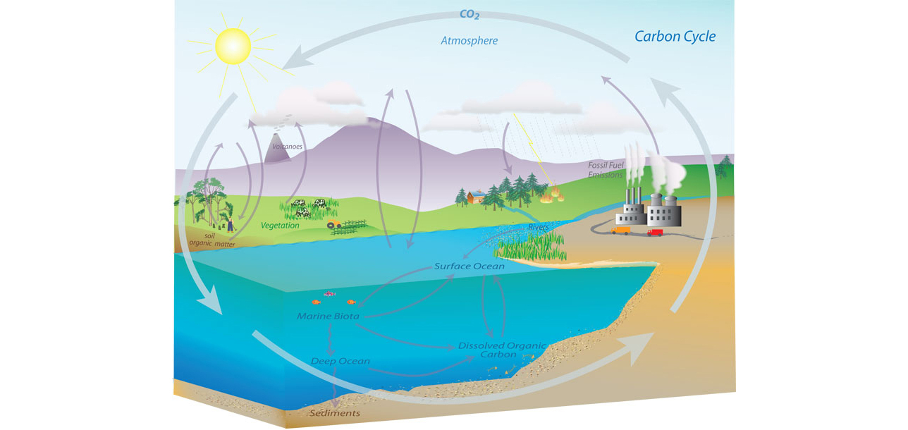
Figure: Representation of the Carbon Cycle from the US National Oceanic and Atmospheric Administration. While everything is interconnected in the system, we can decompose into separate models for atmosphere, ocean, land.

The influence of human activity also needs to be incorporated and modelled so we can make judgments about how to mitigate the effects of global warming.

Figure: The components of a simulation system for climate modelling.

Monolithic System

The classical approach to building these systems was a ‘monolithic system.’ Built in a similar way to the successful applications software such as Excel or Word, or large operating systems, a single code base was constructed. The complexity of such code bases run to many lines.

In practice, shared dynamically linked libraries may be used for aspects such as user interface, or networking, but the software often has many millions of lines of code. For example, the Microsoft Office suite is said to contain over 30 million lines of code.

Figure: A potential path of models in a machine learning system.

Service Oriented Architecture

Such software is not only difficult to develop, but also to scale when computation demands increase. For example, Amazon’s original website software (called Obidos) was a monolithic design but by the early noughties it was becoming difficult to sustain and maintain. The software was phased out in 2006 to be replaced by a modularized software known as a ‘service-oriented architecture.’

In Service Oriented Architecture, or “Software as a Service” the idea is that code bases are modularized and communicate with one another using network requests. A standard approach is to use a REST API. So, rather than a single monolithic code base, the code is developed with individual services that handle the different requests.

The simulation software is turned inside out to expose the individual components to the operator.

Figure: A potential path of models in a machine learning system.

This is the landscape we now find ourselves in for software development. In practice, each of these services is often ‘owned’ and maintained by an individual team. The team is judged by the quality of their service provision. They work to detailed specifications on what their service should output, what its availability should be and other objectives like speed of response. This allows for conditional independence between teams and for faster development.

One question is to what extent is the same approach possible/desirable for scientific models? The components we listed above are already separated and often run independently. But those components themselves are made up of other sub-components that could also be exposed in a similar manner to software-as-a-service, giving us the notion of “simulation as a service.”

Emulation

[edit]

Figure: A statistical emulator is a system that reconstructs the simulation with a statistical model.

A statistical emulator is a data-driven model that learns about the underlying simulation. Importantly, learns with uncertainty, so it ‘knows what it doesn’t know.’ In practice, we can call the emulator in place of the simulator. If the emulator ‘doesn’t know,’ it can call the simulator for the answer.

Figure: A statistical emulator is a system that reconstructs the simulation with a statistical model. As well as reconstructing the simulation, a statistical emulator can be used to correlate with the real world.

As well as reconstructing an individual simulator, the emulator can calibrate the simulation to the real world, by monitoring differences between the simulator and real data. This allows the emulator to characterise where the simulation can be relied on, i.e. we can validate the simulator.

Similarly, the emulator can adjudicate between simulations. This is known as multi-fidelity emulation. The emulator characterizes which emulations perform well where.

If all this modelling is done with judiscious handling of the uncertainty, the computational doubt, then the emulator can assist in desciding what experiment should be run next to aid a decision: should we run a simulator, in which case which one, or should we attempt to acquire data from a real world intervention.

Deep Emulation

[edit]

Figure: A potential path of models in the emulation of a simulation system.

As a solution we can use of emulators. When constructing an ML system, software engineers, ML engineers, economists and operations researchers are explicitly defining relationships between variables of interest in the system. That implicitly defines a joint distribution, $p(\mathbf{ y}^*, \mathbf{ y})$. In a decomposable system any sub-component may be defined as $p(\mathbf{ y}_\mathbf{i}|\mathbf{ y}_\mathbf{j})$ where $\mathbf{ y}_\mathbf{i}$ and $\mathbf{ y}_\mathbf{j}$ represent sub-sets of the full set of variables $\left\{\mathbf{ y}^*, \mathbf{ y}\right\}$. In those cases where the relationship is deterministic, the probability density would collapse to a vector-valued deterministic function, $\mathbf{ f}_\mathbf{i}\left(\mathbf{ y}_\mathbf{j}\right)$.

Inter-variable relationships could be defined by, for example a neural network (machine learning), an integer program (operational research), or a simulation (supply chain). This makes probabilistic inference in this joint density for real world systems is either very hard or impossible.

Emulation is a form of meta-modelling: we construct a model of the model. We can define the joint density of an emulator as $s(\mathbf{ y}*, \mathbf{ y})$, but if this probability density is to be an accurate representation of our system, it is likely to be prohibitively complex. Current practice is to design an emulator to deal with a specific question. This is done by fitting an ML model to a simulation from the the appropriate conditional distribution, $p(\mathbf{ y}_\mathbf{i}|\mathbf{ y}_\mathbf{j})$, which is intractable. The emulator provides an approximated answer of the form $s(\mathbf{ y}_\mathbf{i}|\mathbf{ y}_\mathbf{j})$. Critically, an emulator should incorporate its uncertainty about its approximation. So the emulator answer will be less certain than direct access to the conditional $p(\mathbf{ y}_i|\mathbf{ y}_j)$, but it may be sufficiently confident to act upon. Careful design of emulators to answer a given question leads to efficient diagnostics and understanding of the system. But in a complex interacting system an exponentially increasing number of questions can be asked. This calls for a system of automated construction of emulators which selects the right structure and redeploys the emulator as necessary. Rapid redeployment of emulators could exploit pre-existing emulators through transfer learning.

Automatically deploying these families of emulators for full system understanding is highly ambitious. It requires advances in engineering infrastructure, emulation, and Bayesian optimization. However, the intermediate steps of developing this architecture also allow for automated monitoring of system accuracy and fairness. This facilitates AutoML on a component-wise basis which we can see as a simple implementation of AutoAI. The proposal is structured so that despite its technical ambition there is a smooth ramp of benefits to be derived across the program of work.

In Applied Mathematics, the field studying these techniques is known as uncertainty quantification. The new challenge is the automation of emulator creation on demand to answer questions of interest and facilitate the system design, i.e. AutoAI through BSO.

At design stage, any AI task could be decomposed in multiple ways. Bayesian system optimization will assist both in determining the large-scale system design through exploring different decompositions and in refinement of the deployed system.

So far, most work on emulators has focused on emulating a single component. Automated deployment and maintenance of ML systems requires networks of emulators that can be deployed and redeployed on demand depending on the question of interest. Therefore, the technical innovations we require are in the mathematical composition of emulator models (Damianou and Lawrence, 2013; Perdikaris et al., 2017). Different chains of emulators will need to be rapidly composed to make predictions of downstream performance. This requires rapid retraining of emulators and propagation of uncertainty through the emulation pipeline a process we call deep emulation.

This structural learning allows us to associate data with the relevant layer of the model, rather than merely on the leaf nodes of the output model. When deploying the deep Gaussian process as an emulator, this allows for the possibility of learning the structure of the different component parts of the underlying system. This should aid the user in determining the ideal system decomposition.

Figure: A potential path of models in a machine learning system.

Figure: A potential path of models in the emulation of a simulation system.

Conclusions

The particular circumstances of the Covid-19 pandemic have highlighted the challenges of integrating scientific ideas to answer policy questions. In this talk, we’ve given a formal introduction to the problem, the difficulty of communicating between individuals (particularly from different domains) and reviewed the ideas and solutions we used in the Delve initiative.

Recommendations from the DELVE Data report suggest that more effort needs to be placed into working in this manner in normal circumstances, so that when an emergency occurs we are better prepared to deal with the questions we face.

When we combine these difficult challenges with complex models, we need to put more effort into decomposing our models so that they may be calibrated and re-integrated at appropriate fidelities.

Thanks!

For more information on these subjects and more you might want to check the following resources.

References

Chater, N., 2019. The mind is flat. Penguin.

Damianou, A., Lawrence, N.D., 2013. Deep Gaussian processes. pp. 207–215.

Heider, F., 1958. The psychology of interpersonal relations. John Wiley.

Kahneman, D., 2011. Thinking fast and slow.

Perdikaris, P., Raissi, M., Damianou, A., Lawrence, N.D., Karnidakis, G.E., 2017. Nonlinear information fusion algorithms for data-efficient multi-fidelity modelling. Proc. R. Soc. A 473. https://doi.org/10.1098/rspa.2016.0751

The DELVE Initiative, 2020a. Data readiness: Lessons from an emergency. The Royal Society.

The DELVE Initiative, 2020f. Economic aspects of the COVID-19 crisis in the UK. The Royal Society.

The DELVE Initiative, 2020b. Face masks for the general public. The Royal Society.

The DELVE Initiative, 2020d. Scoping report on hospital and health care acquisition of COVID-19 and its control. The Royal Society.

The DELVE Initiative, 2020e. Balancing the risks of pupils returning to schools. The Royal Society.

The DELVE Initiative, 2020c. Test, trace, isolate. The Royal Society.

The DELVE Initiative, 2020g. SARS-CoV-2 vaccine development & implementation; scenarios, options, key decisions. The Royal Society.

Disraeli is attributed this quote by Mark Twain.↩︎