AI for Science
Abstract
AI is changing how science is practiced: from data analysis and surrogate modelling to the use of large, general-purpose models as scientific assistants that can read, write, code, and coordinate work.
This opening lecture frames the workshop’s core questions as questions about where knowledge lives, what we mean by understanding, and how we preserve scientific agency when useful models are not fully intelligible. We’ll build on Popper/Kuhn perspectives on scientific progress, and outline questions for an AI-for-science “playbook” with particular focus on the ideas of tacit knowledge and “agentic debt.”
Rabbits and Headlights
Sometimes it’s useful to look back and see what we were thinking at a particular time. Manning (2015) covered the incoming deep learning tsunami.
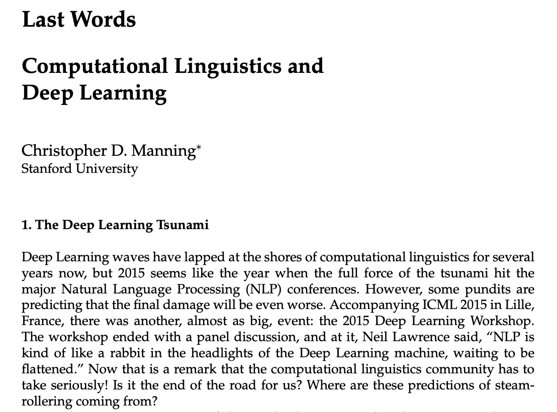

Figure: Chris Manning quoting me in 2015 on the coming wave in Natural Language Processing in Manning (2015).
The quote comes from the Deep Learning Workshop at 2015 ICML. For a transcript see this page: https://the-atomic-human.ai/archive/icml-deep-learning-workshop-panel/.
A Provocation
With that in mind perhaps it’s worth delivering the following provocation.
Science is kind of like a rabbit in the headlights of the Deep Learning Machine waiting to be flattened.
Or are we actually already in the middle of the flood. And if so, where is the high ground?
Questions
As a way of triggering reflection for this workshop we thought to start with three questions. They are:
- Where do scientific paradigms live as knowledge moves from books/equations into code, simulators, and large models?
- What role should human understanding and agency play when we can use models we don’t fully understand?
- What’s an emerging playbook for AI-for-science* and what tools will we depend on?
To start exploring we’ll look at some ideas from the philosophy of science, starting with Thomas Kuhn.
The Structure of Scientific Revolutions

Figure: The Structure of Scientific Revolutions by Thomas S. Kuhn suggests scientific paradigms are recorded in books (Kuhn, 1962).
Kuhn was a historian of science and a philosopher who suggested that the sociology of science has two principal components to it. His idea is that “normal science” operates within a paradigm That paradigm is defined by books which encode our best understanding. An example of a paradigm is Newtonian mechanics, or another example would be the geocentric view of the Universe. Within a paradigm normal science proceeds by scientists solving the “puzzles” that paradigm sets. A paradigm shift is when the paradigm changes, for example the Corpernican revolution or the introduction of relativity.
The notion of a paradigm shift has also entered common parlance, this reflects the idea that wider human knowledge is also shared and stored, less ormally than scientific knowledge, but still with a dependence on our information infrastructure.
The digital computer has brought a fundamental change in the nature of that information infrastructure. By moving information faster the modern information infrastructure is dominated not by the book, but by the machine. This brings challenges for managing and controlling this information infrastructure.
See Lawrence (2024) Kuhn, Thomas: The Structure of Scientific Revolutions p. 295–299.
Kuhn’s idea that science iterates between normal science (or puzzle solving) and paradigm shifts which change the fundamental assumptions that underpin our scientific ideas. Kuhn was writing in 1962 and he argued that at that time our paradigm was stored in text books. Even before the advent of AI, our modern information infrastructure has shifted, to the extent that one can argue that today our paradigm is (also) stored in computers, through simulations, databases etc..
This leads to a provocation as to whether we are experiencing a paradigm shift in science, or more structurally a paradigm shift in the way our scientific paradigms are stored and shared. A fundamental change in the underpinning information infrastructure.
Conjectures and Refutations
Figure: Conjectures and Refutations by Karl Popper presents his philosophy of science based on falsification.
In “Conjectures and Refutations” (Popper, 1963), Popper elaborates on his philosophy of science, arguing that scientific knowledge progresses through bold conjectures that are then subjected to rigorous attempts at refutation. He contrasts this with verification-based approaches, arguing that no amount of confirmatory evidence can prove a universal theory, but a single counter-example can disprove it.
This philosophy of falsificationism suggests that scientists should actively try to disprove their theories rather than seek confirming evidence. For Popper, what makes a theory scientific is not its ability to be verified, but its ability to be falsified - it must make predictions that could potentially be proven wrong.
These ideas have profound implications for how we understand scientific progress and the scientific method. It implies science isn’t an activity of individuals, it is necessarily a community effort.
See Lawrence (2024) Popper, Karl: Conjectures and Refutations p. 327,328.
Qualitative vs Quantitative
Historically questions can be split into two types. Qualitative questions and quantitative questions. Arguably most of the questions we truly care about are qualitiative, “How can I live a happier life?” “How can I do more good in the world?” “Will this drug make me healthier?” But in practice the questions we answer scientifically tend to be quantitative. “Which jobs have the highest income?” “What is the GDP/capita of Kenya?” “Does this drug give an average life extension of greater than 6 months?”
This new generation of AI seems in some ways to bridge the qualitative/quantitive gap. Firstly, language can now be used directly as data, perhaps allowing us to bring a more quantitative approach to what were formerly qualitative questions. But secondly traditional techniques in social science that are based on interviews or transcripts (e.g. grounded theory) could be made more scalable with the use of AI technologies. For example, automatic transcription and/or assisted coding.
Coding and Creatives
Just to contextualise for a moment, imagine we have stepped back to that ICML workshop 11 years ago where I made that quote. I think one thing that would have suprised us is the effect of that Tsunami. Up until last year at least it feels like the main direct societal effect was on coding and creatives. Although I have some sense of why that is (you might have your own answers), I think I would have found that very difficult to predict, or indeed to have imagined any technology that has a major effect on those two areas.
Even before modern AI, specialisation plus scale meant no one could hold the whole map of science in their head. Today, tools can make cross-field exploration easier: you can ask a model to summarise, translate notation, find relevant papers, draft code, or suggest plausible mechanisms. But the failure mode is also cross-field: confident-sounding claims without the embodied judgement that comes from living inside a discipline (Kwon, 2025; Narayanan and Kapoor, 2025; O’Grady, 2025).
This framing is meant to reduce the “AI for science” hype conflation by separating three different questions we often mix together. First, what can a model technically do (task capability)? Second, where in scientific practice does it add value (workflow need)? Third, what constraints make deployment viable in a given field (context constraints)? The same model can look transformative in one workflow and marginal in another; likewise, a method that works in one domain can fail in another because validation, latency, compute, or uncertainty tolerance differ. The practical aim is better matching: align capabilities to scientific questions and local constraints, rather than assuming a general model gives general scientific benefit.
The “science gap” is the distance between statistical competence and scientific understanding. Pattern matching can produce accurate predictions, but scientific reasoning usually asks for mechanistic structure: what would happen under interventions, out-of-distribution conditions, or policy-relevant counterfactuals. In practice this leads to a guess-and-verify loop: models generate candidates, experiments filter them. That can still be useful science, but it shifts where understanding lives and where cost sits. The key point here is not that prediction is bad, but that prediction and explanation are different epistemic products, and we should be explicit about which one a workflow is optimising for.
These three priorities are an agenda for making AI more scientific. Causality asks whether models can support intervention and policy reasoning, not only retrospective fit. Abstraction asks whether AI can help discover the right intermediate representations across scales, where many scientific breakthroughs occur. Simulation asks how to combine mechanistic structure with learned components so we retain physical plausibility while gaining flexibility and efficiency. Together they move us from “high-performing predictor” toward “scientific instrument”: a system that is useful, interrogable, and bounded by clear validity conditions.
To Tim
To Tim
- Perhaps: “what is science?” as prediction, explanation, and control.
- Perhaps: where control/RL intuitions shift how we evaluate models.
- Perhaps: how model classes connect (equations, effective statistical models, ML systems).
What is science for?
- Prediction: what will happen?
- Explanation: why does it happen?
- Control/Design: how do we intervene to get desired outcomes?
- Different fields weight these differently; AI changes the balance.
Model types in science
- Mechanistic models: equations from domain theory.
- Effective/statistical models: coarse-grained abstractions (e.g., stat mech style summaries).
- Learned models: ML/DL surrogates and pattern extractors.
- Practice is hybrid: compose all three with clear verification boundaries.
In the first wave of ML in science we’ve seen the increasing use of ML/statistical models for prediction. Here we fit a function \(\f_\theta\) on the basis of a large data set or a simulation (statistical emulation/surrogate modelling). This allows us to explore that simulation or data through the model we’ve created and the predictions it makes.
Examples include AlphaFold and data-driven weather forecasting systems (Allen et al., 2025; Jumper et al., 2021), as well as materials discovery (Merchant et al., 2023).
Over the last decade we’ve seen the emergence of new “generalist” or foundation models. Starting with image recognition we found we could fine-tune models trained on one image data set and transfer their capabilities to other data sets.
The same thing proved true of language once we’d developed transformer architectures and large language models.
A “Polymathic”-style model trained on differential equations is interesting because it shifts the discussion. In many domains we can’t even agree what the canonical “ground truth” representation is; in physics we often can. That creates a rare opportunity: we can evaluate generalisation against known structure, probe failure modes, and ask whether the learned representations correspond to anything mechanistic or merely operationally effective.
At the extreme end of fine tuning these large language models can now be directed by prompting, or setting a context. These models are built to emulate human intelligence by reconstructing what humans might have said. They are augmented by code and maths problems in a process I think of as “vulcanisation”1.
Break (15 mins)
- Return for delegation, tacit knowledge, and verification boundaries.
Suggested break after Tim’s first block. Re-start by recapping the prediction/explanation/control lens and move into accountability.
The Unreasonable Effectiveness of Orchestration
The most recent trend is orchestration of these different parts through chat interfaces. Unsurprisingly, since these models are emulating a form of human intelligence, like humans they are more effective when working in a team. But these teams also are given tool calling abilities which allows them rapid access to the information infrastructure. That is leading to the unreasonable effectiveness of agents.
That means that an additional pattern is emerging, its no longer just prediction2 but and this raises new questions about our processes in Science.
What are we Delegating?
A distinction that I don’t think was relevant for Popper when writing in 1963 was whether it matters that we understand where conjectures are coming from and we have an intuition about why they might work. At the time it might still have seemed fanciful for a machine to be so high powered that it could be used for (perhaps exhaustively) exploring and generating hypotheses. Whereas today that seems feasible, particularly for orchestrated sytems of agents.
This separation might be summarised as “science as technology” where we are using science to create new materials or drugs that we can empirically show are effective, even if we don’t understand why. Or “science as understanding” where we are building our own understanding through our work.
I think the two will actually co-evolve, but I think the separation is useful when thinking about AI for science because different actions prioritise one versus the other.
Even in the sciene as technology case, society will still require us to have accountability when there are judgment calls. That accountability assumes some understanding. Note that this has already been eroded to some extent. Think, for example, of a computational epidemiologist in the Covid19 pandemic being asked to explain what their model includes (such as hotel closures) and what it doesn’t account for (such as facemasks!).
We might not have data, but we do have arithmetic
This leads to a phenomena I think of as “agentic debt.” And the related phenomenon of “scientific or intellectual debt.”
Intellectual Debt

Figure: Jonathan Zittrain’s term to describe the challenges of explanation that come with AI is Intellectual Debt.
In the context of machine learning and complex systems, Jonathan Zittrain has coined the term “Intellectual Debt” to describe the challenge of understanding what you’ve created. In the ML@CL group we’ve been foucssing on developing the notion of a data-oriented architecture to deal with intellectual debt (Cabrera et al., 2023).
Zittrain points out the challenge around the lack of interpretability of individual ML models as the origin of intellectual debt. In machine learning I refer to work in this area as fairness, interpretability and transparency or FIT models. To an extent I agree with Zittrain, but if we understand the context and purpose of the decision making, I believe this is readily put right by the correct monitoring and retraining regime around the model. A concept I refer to as “progression testing.” Indeed, the best teams do this at the moment, and their failure to do it feels more of a matter of technical debt rather than intellectual, because arguably it is a maintenance task rather than an explanation task. After all, we have good statistical tools for interpreting individual models and decisions when we have the context. We can linearise around the operating point, we can perform counterfactual tests on the model. We can build empirical validation sets that explore fairness or accuracy of the model.
See Lawrence (2024) intellectual debt p. 84, 85, 349, 365.
Technical Debt
In computer systems the concept of technical debt has been surfaced by authors including Sculley et al. (2015). It is an important concept, that I think is somewhat hidden from the academic community, because it is a phenomenon that occurs when a computer software system is deployed.
Separation of Concerns
To construct such complex systems an approach known as “separation of concerns” has been developed. The idea is that you architect your system, which consists of a large-scale complex task, into a set of simpler tasks. Each of these tasks is separately implemented. This is known as the decomposition of the task.
This is where Jonathan Zittrain’s beautifully named term “intellectual debt” rises to the fore. Separation of concerns enables the construction of a complex system. But who is concerned with the overall system?
Technical debt is the inability to maintain your complex software system. Intellectual debt is the inability to explain your software system.
It is right there in our approach to software engineering. “Separation of concerns” means no one is concerned about the overall system itself.
See Lawrence (2024) separation of concerns p. 84-85, 103, 109, 199, 284, 371.
See Lawrence (2024) intellectual debt p. 84-85, 349, 365, 376.
Agentic Debt
Agentic AI could pay down the technical debt and intellectual debt that plauges our deployment of complex systems. But in doing so it could create a new form of debt: agentic debt.
Agentic debt is the “new debt” introduced by systems that can act: the accrued risk and cost of operating delegated workflows without crisp boundaries. Unlike technical debt, e.g. emerging from engineering shortcuts, and intellectual debt emerging from (well engineered) complex systems, agentic debt is about unsafe or illegible delegation. Who (or what) can cause what action, on what evidence, with what recovery path?
The answers differ when our understanding of the underlying physics improves: think of Navier Stokes simulations, or quantum field theory for chemical bonding vs economic models or “social digital twins.”
What is the judgment layer for AI in Science? How do we maintain accountability when we have delegated the process of discovery to agents?
We can mean different things by understanding:
- Operational understanding: can I use it safely and know when it fails?
- Mechanistic understanding: do I have an interpretable causal/mechanistic story?
- Paradigm understanding: can the community reproduce, contest, and extend it?
- Social understanding: are the ideas understood in the wider public and other fields? (Lawrence, 2024)
With increasing use of computation in science we could argue that there’s a shift from mechanistic to operational understanding. But if AI tools are judiciously deployed we could argue that they could support a shift to better understanding of our own paradigms and broader social understanding.
These different forms of understanding enable different forms of individual, institutional and social accountability. The machines cannot participate in this social accountability in the same way we do because they are not socially vested.
Institutional tacit knowledge
This motivates an emulsion metaphor: organisations are a stable mixture of automatable routines and irreducible human context. In current institutions, the interface between these routine decisions and the judgment is mixed, like an emulsion. When we replace these decisions with orchestrated agents without understanding the judgment interventions we accumulate agentic debt. Paying down agentic debt means extracting the tacit judgment layer into explicit policies, evidence requirements, and reversible action boundaries.
The Information Infrastructure
Embodiment Factors: Walking vs Light Speed
Imagine human communication as moving at walking pace. The average person speaks about 160 words per minute, which is roughly 2000 bits per minute. If we compare this to walking speed, roughly 1 m/s we can think of this as the speed at which our thoughts can be shared with others.
Compare this to machines. When computers communicate, their bandwidth is 600 billion bits per minute. Three hundred million times faster than humans or the equiavalent of \(3 \times 10 ^{8}\). In twenty minutes we could be a kilometer down the road, where as the computer can go to the Sun and back again..
This difference is not just only about speed of communication, but about embodiment. Our intelligence is locked in by our biology: our brains may process information rapidly, but our ability to share those thoughts is limited to the slow pace of speech or writing. Machines, in comparison, seem able to communicate their computations almost instantaneously, anywhere.
So, the embodiment factor is the ratio between the time it takes to think a thought and the time it takes to communicate it. For us, it’s like walking; for machines, it’s like moving at light speed. This difference means that most direct comparisons between human and machine need to be carefully made. Because for humans not the size of our communication bandwidth that counts, but it’s how we overcome that limitation..
New Flow of Information
Classically the field of statistics focused on mediating the relationship between the machine and the human. Our limited bandwidth of communication means we tend to over-interpret the limited information that we are given, in the extreme we assign motives and desires to inanimate objects (a process known as anthropomorphizing). Much of mathematical statistics was developed to help temper this tendency and understand when we are valid in drawing conclusions from data.
Figure: The trinity of human, data, and computer, and highlights the modern phenomenon. The communication channel between computer and data now has an extremely high bandwidth. The channel between human and computer and the channel between data and human is narrow. New direction of information flow, information is reaching us mediated by the computer. The focus on classical statistics reflected the importance of the direct communication between human and data. The modern challenges of data science emerge when that relationship is being mediated by the machine.
Data science brings new challenges. In particular, there is a very large bandwidth connection between the machine and data. This means that our relationship with data is now commonly being mediated by the machine. Whether this is in the acquisition of new data, which now happens by happenstance rather than with purpose, or the interpretation of that data where we are increasingly relying on machines to summarize what the data contains. This is leading to the emerging field of data science, which must not only deal with the same challenges that mathematical statistics faced in tempering our tendency to over interpret data but must also deal with the possibility that the machine has either inadvertently or maliciously misrepresented the underlying data.
See Lawrence (2024) topography, information p. 34-9, 43-8, 57, 62, 104, 115-16, 127, 140, 192, 196, 199, 291, 334, 354-5. See Lawrence (2024) anthropomorphization (‘anthrox’) p. 30-31, 90-91, 93-4, 100, 132, 148, 153, 163, 216-17, 239, 276, 326, 342.
HAM
The Human-Analogue Machine or HAM therefore provides a route through which we could better understand our world through improving the way we interact with machines.
Figure: The trinity of human, data, and computer, and highlights the modern phenomenon. The communication channel between computer and data now has an extremely high bandwidth. The channel between human and computer and the channel between data and human is narrow. New direction of information flow, information is reaching us mediated by the computer. The focus on classical statistics reflected the importance of the direct communication between human and data. The modern challenges of data science emerge when that relationship is being mediated by the machine.
The HAM can provide an interface between the digital computer and the human allowing humans to work closely with computers regardless of their understandin gf the more technical parts of software engineering.
Figure: The HAM now sits between us and the traditional digital computer.
Of course this route provides new routes for manipulation, new ways in which the machine can undermine our autonomy or exploit our cognitive foibles. The major challenge we face is steering between these worlds where we gain the advantage of the computer’s bandwidth without undermining our culture and individual autonomy.
See Lawrence (2024) human-analogue machine (HAMs) p. 343-347, 359-359, 365-368.
In Mathematical Context
Terrance Tao’s IMO 2024 talk on machine assitance in maths gives an excellent overview of how ML techniques can be deployed in maths. Well worth watching for additional insight
This is a useful cross-field lens. Mathematics is close to a “gold standard” for verifiability: once formalised, we can check claims mechanically. But much of science lives in tacit practice: what counts as a clean sample, a plausible stratigraphy, a credible causal story, a trustworthy instrument calibration. LLMs are attractive because they can encode and communicate that practice in natural language, but they don’t automatically create verifiable, accountable knowledge. So the design question becomes: where do we draw the verification boundary, and what artefacts do we insist on at that boundary?
This is the need for a practical definition of “accountability” here: not blaming the model, but making the chain legible. For science: who is the author of the claim, what evidence supports it, and what were the decision thresholds? That’s a systems/interface problem, not a model-quality problem.
Technical progress is now moving faster than institutional adaptation. The governance gap is the distance between principles and implementation in day-to-day research practice, including transparency, attribution, and reproducibility. The culture gap reflects incentive systems that still reward disciplinary depth more than the interdisciplinary collaboration AI-for-science needs. The infrastructure gap captures concentration of compute, models, and engineering capacity, which can compromise openness and independence. The narrative gap is about visibility: high-profile corporate successes can obscure the long public investment base that made them possible. The coordination gap recognises that funding, governance, data, and skills policies are often designed in separate silos, even though deployment challenges are coupled.
This playbook is designed as a policy and programme checklist rather than a manifesto. Funding should support both frontier methods and field-embedded deployment teams. Governance should make accountability operational: clear authorship, auditability, and validation norms. Infrastructure policy should widen access to compute and open tools so adoption does not default to a few proprietary stacks. Data policy should focus on trustworthy access, stewardship, and incentives for curation, not just volume. Talent and skills policy should treat explanation, verification, and challenge as core scientific competencies in an AI-mediated workflow. The practical aim is to accelerate adoption while preserving scientific integrity, openness, and public trust.
Developing Science
One of the most important roles of science is developing the next generation of scientists. This is something that Universities do very well. What does this look like in a world where we can rapidly iterate scientific pipelines through llm/tool orchestration?
How do we train the next generation of scientists to explain, verify and challenge. How do we develop their scepticism? How do we convert our tacit knowledge (institutional and individual) about judgement into verification boundaries for AI-for-science systems?
What is the new repository for the paradigm store?
Over to Tim: agents, discovery, specialist tools
Workshop Questions
- Is there an emerging playbook for AI-for-Science?
- Are we converging on a standard recipe, accurate but slow simulators, amortized surrogates, differentiable pipelines, and how do we know when these surrogates truly generalize?
- Can AI grapple with open-ended discovery?
- Beyond supervised prediction, to what extent can current or near-future systems generate meaningful hypotheses, concepts, and research directions?
- What tools do we have, and what tools are missing?
- Which existing AI/ML capabilities are already reshaping scientific practice, and what critical tools (for uncertainty, causality, interpretability, or interfaces) are still absent?
Thanks!
For more information on these subjects and more you might want to check the following resources.
- company: Trent AI
- book: The Atomic Human
- twitter: @lawrennd
- podcast: The Talking Machines
- newspaper: Guardian Profile Page
- blog: http://inverseprobability.com