Deep Gaussian Processes: A Motivation and Introduction
Abstract
Modern machine learning methods have driven significant advances in artificial intelligence, with notable examples coming from Deep Learning, enabling super-human performance in the game of Go and highly accurate prediction of protein folding e.g. AlphaFold. In this talk we look at deep learning from the perspective of Gaussian processes. Deep Gaussian processes extend the notion of deep learning to propagate uncertainty alongside function values. We’ll explain why this is important and show some simple examples.
Introduction
The Fourth Industrial Revolution
The fourth industrial revolution bears the particular hallmark of being the first revolution that has been named before it has happened. This is particularly unfortunate, because it is not in fact an industrial revolution at all. Nor is it necessarily a distinct phenomenon. It is part of a revolution in information, one that goes back to digitisation and the invention of the silicon chip.
Or to put it more precisely, it is a revolution in how information can affect the physical world. The interchange between information and the physical world.
%pip install mlai%pip install notutilsWhat is Machine Learning?
What is machine learning? At its most basic level machine learning is a combination of
\[\text{data} + \text{model} \stackrel{\text{compute}}{\rightarrow} \text{prediction}\]
where data is our observations. They can be actively or passively acquired (meta-data). The model contains our assumptions, based on previous experience. That experience can be other data, it can come from transfer learning, or it can merely be our beliefs about the regularities of the universe. In humans our models include our inductive biases. The prediction is an action to be taken or a categorization or a quality score. The reason that machine learning has become a mainstay of artificial intelligence is the importance of predictions in artificial intelligence. The data and the model are combined through computation.
In practice we normally perform machine learning using two functions. To combine data with a model we typically make use of:
a prediction function a function which is used to make the predictions. It includes our beliefs about the regularities of the universe, our assumptions about how the world works, e.g., smoothness, spatial similarities, temporal similarities.
an objective function a function which defines the cost of misprediction. Typically, it includes knowledge about the world’s generating processes (probabilistic objectives) or the costs we pay for mispredictions (empirical risk minimization).
The combination of data and model through the prediction function and the objective function leads to a learning algorithm. The class of prediction functions and objective functions we can make use of is restricted by the algorithms they lead to. If the prediction function or the objective function are too complex, then it can be difficult to find an appropriate learning algorithm. Much of the academic field of machine learning is the quest for new learning algorithms that allow us to bring different types of models and data together.
A useful reference for state of the art in machine learning is the UK Royal Society Report, Machine Learning: Power and Promise of Computers that Learn by Example.
You can also check my post blog post on What is Machine Learning?.
What does Machine Learning do?
Any process of automation allows us to scale what we do by codifying a process in some way that makes it efficient and repeatable. Machine learning automates by emulating human (or other actions) found in data. Machine learning codifies in the form of a mathematical function that is learnt by a computer. If we can create these mathematical functions in ways in which they can interconnect, then we can also build systems.
Machine learning works through codifing a prediction of interest into a mathematical function. For example, we can try and predict the probability that a customer wants to by a jersey given knowledge of their age, and the latitude where they live. The technique known as logistic regression estimates the odds that someone will by a jumper as a linear weighted sum of the features of interest.
\[ \text{odds} = \frac{p(\text{bought})}{p(\text{not bought})} \]
\[ \log \text{odds} = \beta_0 + \beta_1 \text{age} + \beta_2 \text{latitude}.\] Here \(\beta_0\), \(\beta_1\) and \(\beta_2\) are the parameters of the model. If \(\beta_1\) and \(\beta_2\) are both positive, then the log-odds that someone will buy a jumper increase with increasing latitude and age, so the further north you are and the older you are the more likely you are to buy a jumper. The parameter \(\beta_0\) is an offset parameter, and gives the log-odds of buying a jumper at zero age and on the equator. It is likely to be negative1 indicating that the purchase is odds-against. This is actually a classical statistical model, and models like logistic regression are widely used to estimate probabilities from ad-click prediction to risk of disease.
This is called a generalized linear model, we can also think of it as estimating the probability of a purchase as a nonlinear function of the features (age, lattitude) and the parameters (the \(\beta\) values). The function is known as the sigmoid or logistic function, thus the name logistic regression.
\[ p(\text{bought}) = \sigma\left(\beta_0 + \beta_1 \text{age} + \beta_2 \text{latitude}\right).\] In the case where we have features to help us predict, we sometimes denote such features as a vector, \(\mathbf{ x}\), and we then use an inner product between the features and the parameters, \(\boldsymbol{\beta}^\top \mathbf{ x}= \beta_1 x_1 + \beta_2 x_2 + \beta_3 x_3 ...\), to represent the argument of the sigmoid.
\[ p(\text{bought}) = \sigma\left(\boldsymbol{\beta}^\top \mathbf{ x}\right).\] More generally, we aim to predict some aspect of our data, \(y\), by relating it through a mathematical function, \(f(\cdot)\), to the parameters, \(\boldsymbol{\beta}\) and the data, \(\mathbf{ x}\).
\[ y= f\left(\mathbf{ x}, \boldsymbol{\beta}\right).\] We call \(f(\cdot)\) the prediction function.
To obtain the fit to data, we use a separate function called the objective function that gives us a mathematical representation of the difference between our predictions and the real data.
\[E(\boldsymbol{\beta}, \mathbf{Y}, \mathbf{X})\] A commonly used examples (for example in a regression problem) is least squares, \[E(\boldsymbol{\beta}, \mathbf{Y}, \mathbf{X}) = \sum_{i=1}^n\left(y_i - f(\mathbf{ x}_i, \boldsymbol{\beta})\right)^2.\]
If a linear prediction function is combined with the least squares objective function then that gives us a classical linear regression, another classical statistical model. Statistics often focusses on linear models because it makes interpretation of the model easier. Interpretation is key in statistics because the aim is normally to validate questions by analysis of data. Machine learning has typically focussed more on the prediction function itself and worried less about the interpretation of parameters, which are normally denoted by \(\mathbf{w}\) instead of \(\boldsymbol{\beta}\). As a result non-linear functions are explored more often as they tend to improve quality of predictions but at the expense of interpretability.
Deep Learning
Classical statistical models and simple machine learning models have a great deal in common. The main difference between the fields is philosophical. Machine learning practitioners are typically more concerned with the quality of prediciton (e.g. measured by ROC curve) while statisticians tend to focus more on the interpretability of the model and the validity of any decisions drawn from that interpretation. For example, a statistical model may be used to validate whether a large scale intervention (such as the mass provision of mosquito nets) has had a long term effect on disease (such as malaria). In this case one of the covariates is likely to be the provision level of nets in a particular region. The response variable would be the rate of malaria disease in the region. The parmaeter, \(\beta_1\) associated with that covariate will demonstrate a positive or negative effect which would be validated in answering the question. The focus in statistics would be less on the accuracy of the response variable and more on the validity of the interpretation of the effect variable, \(\beta_1\).
A machine learning practitioner on the other hand would typically denote the parameter \(w_1\), instead of \(\beta_1\) and would only be interested in the output of the prediction function, \(f(\cdot)\) rather than the parameter itself. The general formalism of the prediction function allows for non-linear models. In machine learning, the emphasis on prediction over interpretability means that non-linear models are often used. The parameters, \(\mathbf{w}\), are a means to an end (good prediction) rather than an end in themselves (interpretable).
DeepFace
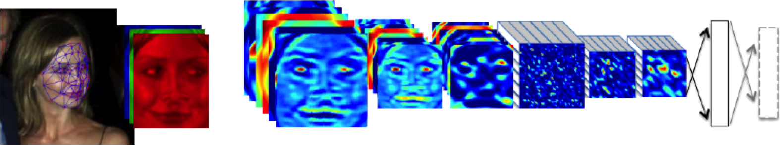

Figure: The DeepFace architecture (Taigman et al., 2014), visualized through colors to represent the functional mappings at each layer. There are 120 million parameters in the model.
The DeepFace architecture (Taigman et al., 2014) consists of layers that deal with translation invariances, known as convolutional layers. These layers are followed by three locally-connected layers and two fully-connected layers. Color illustrates feature maps produced at each layer. The neural network includes more than 120 million parameters, where more than 95% come from the local and fully connected layers.
Deep Learning as Pinball
Figure: Deep learning models are composition of simple functions. We can think of a pinball machine as an analogy. Each layer of pins corresponds to one of the layers of functions in the model. Input data is represented by the location of the ball from left to right when it is dropped in from the top. Output class comes from the position of the ball as it leaves the pins at the bottom.
Sometimes deep learning models are described as being like the brain, or too complex to understand, but one analogy I find useful to help the gist of these models is to think of them as being similar to early pin ball machines.
In a deep neural network, we input a number (or numbers), whereas in pinball, we input a ball.
Think of the location of the ball on the left-right axis as a single number. Our simple pinball machine can only take one number at a time. As the ball falls through the machine, each layer of pins can be thought of as a different layer of ‘neurons.’ Each layer acts to move the ball from left to right.
In a pinball machine, when the ball gets to the bottom it might fall into a hole defining a score, in a neural network, that is equivalent to the decision: a classification of the input object.
An image has more than one number associated with it, so it is like playing pinball in a hyper-space.
Figure: At initialization, the pins, which represent the parameters of the function, aren’t in the right place to bring the balls to the correct decisions.
Figure: After learning the pins are now in the right place to bring the balls to the correct decisions.
Learning involves moving all the pins to be in the correct position, so that the ball ends up in the right place when it’s fallen through the machine. But moving all these pins in hyperspace can be difficult.
In a hyper-space you have to put a lot of data through the machine for to explore the positions of all the pins. Even when you feed many millions of data points through the machine, there are likely to be regions in the hyper-space where no ball has passed. When future test data passes through the machine in a new route unusual things can happen.
Adversarial examples exploit this high dimensional space. If you have access to the pinball machine, you can use gradient methods to find a position for the ball in the hyper space where the image looks like one thing, but will be classified as another.
Probabilistic methods explore more of the space by considering a range of possible paths for the ball through the machine. This helps to make them more data efficient and gives some robustness to adversarial examples.
Deep Neural Network
%pip install daftFigure: A deep neural network. Input nodes are shown at the bottom. Each hidden layer is the result of applying an affine transformation to the previous layer and placing through an activation function.
Mathematically, each layer of a neural network is given through computing the activation function, \(\phi(\cdot)\), contingent on the previous layer, or the inputs. In this way the activation functions, are composed to generate more complex interactions than would be possible with any single layer. \[ \begin{align*} \mathbf{ h}_{1} &= \phi\left(\mathbf{W}_1 \mathbf{ x}\right)\\ \mathbf{ h}_{2} &= \phi\left(\mathbf{W}_2\mathbf{ h}_{1}\right)\\ \mathbf{ h}_{3} &= \phi\left(\mathbf{W}_3 \mathbf{ h}_{2}\right)\\ f&= \mathbf{ w}_4 ^\top\mathbf{ h}_{3} \end{align*} \]
AlphaGo
In January 2016, the UK company DeepMind’s machine learning system AlphaGo won a challenge match in which it beat the world champion Go player, Lee Se-Deol.
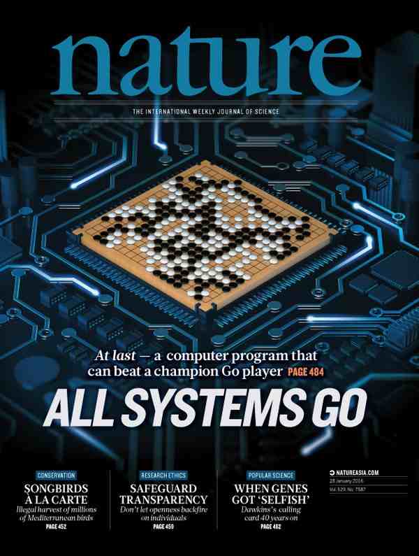
Figure: AlphaGo’s win made the front cover of the journal Nature.
Go is a board game that is known to be over 2,500 years old. It is considered challenging for computer systems becaue of its branching factor: the number of possible moves that can be made at a given board postion. The branching factor of Chess is around 35. The branching factor of Go is around 250. This makes Go less susceptible to exhaustive search techniques which were a foundation of DeepBlue, the chess machine that was able to win against Gary Kasparov in 1997. As a result, many commentators predicted that Go was out of the reach of contemporary AI systems, with some predicting that beating the world champion wouldn’t occur until 2025.
Figure: The AlphaGo documentary tells the story of the tournament between Lee Se-dol and AlphaGo.
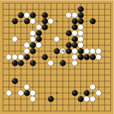
While exhaustive search was beyond the reach of computer systems, they combined stochastic search of the game tree with neural networks. But when training those neural networks vast quantities of data and game play were used. I wrote more about this at the time in the Guardian article “Guardian article on Google AI versus the Go grandmaster.”
However, despite the many millions of matches that AlphaGo had played, Lee Sedol managed to find a board position that was distinct from anything AlphaGo had seen before. Within the high dimensional pinball machine that made up AlphaGo’s decision making systems, Lee Sedol found a niche, an Achillean chink in AlphaGo’s armour. He found a path through the neural network where no data had every been before. He found a location in feature space “where there be dragons.” A space where the model had not seen data before and one where it became confused.
|
|
This is a remarkable achievement, a human, with far less experience than the machine of the game, was able to outplay by placing the machine in an unfamiliar situation. In honour of this achievements, I like to call these voids in the machines understanding “Sedolian voids.”
Uber ATG
Unfortunately, such Sedolian voids are not constrained to game playing machines. On March 18th 2018, just two years after AlphaGo’s victory, the Uber ATG self-driving vehicle killed a pedestrian in Tuscson Arizona. The neural networks that were trained on pedestrian detection did not detect Elaine because she was pushing a bicycle, laden with her bags, across the highway.2 This situation represented a Sedolian void for the neural network, and it failed to stop the car.
Figure: A vehicle operated by Uber ATG was involved in a fatal crash when it killed pedestrian Elaine Herzberg, 49.
Characterising the regions where this is happening for these models remains an outstanding challenge.
In practice, we normally also have uncertainty associated with these functions. Uncertainty in the prediction function arises from
- scarcity of training data and
- mismatch between the set of prediction functions we choose and all possible prediction functions.
There are also challenges around specification of the objective function, but for we will save those for another day. For the moment, let us focus on the prediction function.
Bayesian Inference by Rejection Sampling
One view of Bayesian inference is to assume we are given a mechanism for generating samples, where we assume that mechanism is representing an accurate view on the way we believe the world works.
This mechanism is known as our prior belief.
We combine our prior belief with our observations of the real world by discarding all those prior samples that are inconsistent with our observations. The likelihood defines mathematically what we mean by inconsistent with the observations. The higher the noise level in the likelihood, the looser the notion of consistent.
The samples that remain are samples from the posterior.
This approach to Bayesian inference is closely related to two sampling techniques known as rejection sampling and importance sampling. It is realized in practice in an approach known as approximate Bayesian computation (ABC) or likelihood-free inference.
In practice, the algorithm is often too slow to be practical, because most samples will be inconsistent with the observations and as a result the mechanism must be operated many times to obtain a few posterior samples.
However, in the Gaussian process case, when the likelihood also assumes Gaussian noise, we can operate this mechanism mathematically, and obtain the posterior density analytically. This is the benefit of Gaussian processes.
First, we will load in two python functions for computing the covariance function.
Next, we sample from a multivariate normal density (a multivariate Gaussian), using the covariance function as the covariance matrix.
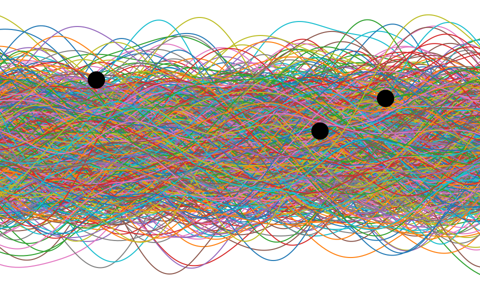
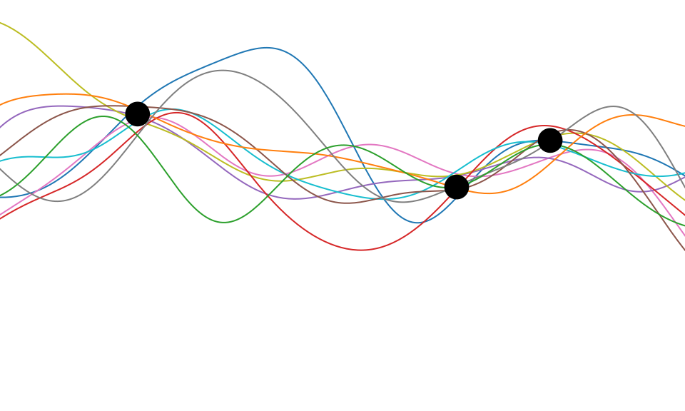
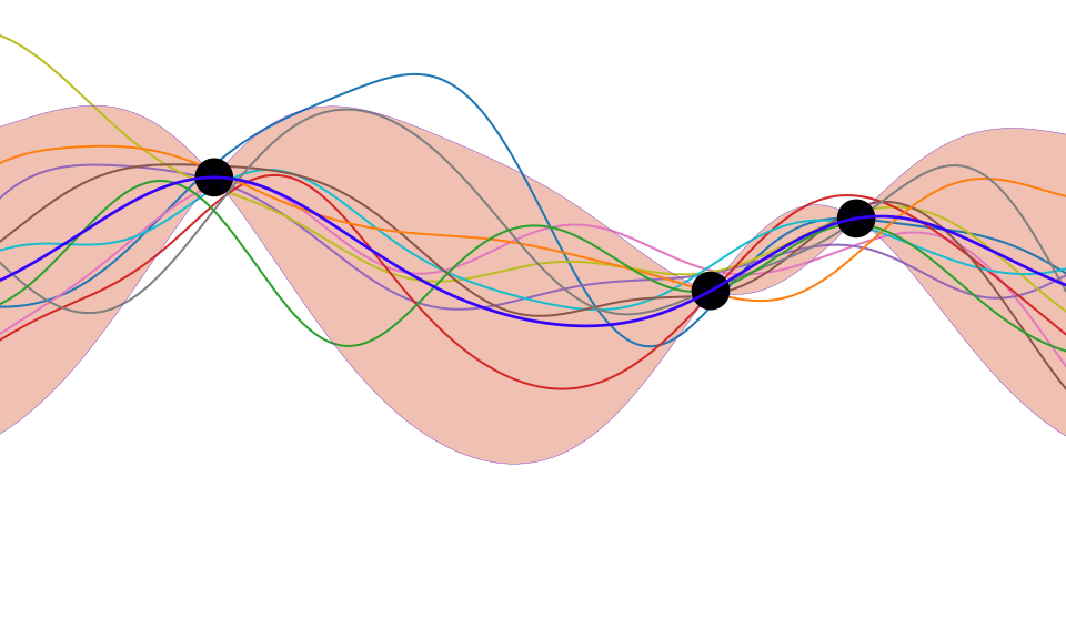
Figure: One view of Bayesian inference is we have a machine for generating samples (the prior), and we discard all samples inconsistent with our data, leaving the samples of interest (the posterior). This is a rejection sampling view of Bayesian inference. The Gaussian process allows us to do this analytically by multiplying the prior by the likelihood.
Structure of Priors
Even in the early days of Gaussian processes in machine learning, it was understood that we were throwing something fundamental away. This is perhaps captured best by David MacKay in his 1997 NeurIPS tutorial on Gaussian processes, where he asked “Have we thrown out the baby with the bathwater?” The quote below is from his summarization paper.
According to the hype of 1987, neural networks were meant to be intelligent models which discovered features and patterns in data. Gaussian processes in contrast are simply smoothing devices. How can Gaussian processes possibly replace neural networks? What is going on?
MacKay (n.d.)
Overfitting
One potential problem is that as the number of nodes in two adjacent layers increases, the number of parameters in the affine transformation between layers, \(\mathbf{W}\), increases. If there are \(k_{i-1}\) nodes in one layer, and \(k_i\) nodes in the following, then that matrix contains \(k_i k_{i-1}\) parameters, when we have layer widths in the 1000s that leads to millions of parameters.
One proposed solution is known as dropout where only a sub-set of the neural network is trained at each iteration. An alternative solution would be to reparameterize \(\mathbf{W}\) with its singular value decomposition. \[ \mathbf{W}= \mathbf{U}\boldsymbol{ \Lambda}\mathbf{V}^\top \] or \[ \mathbf{W}= \mathbf{U}\mathbf{V}^\top \] where if \(\mathbf{W}\in \Re^{k_1\times k_2}\) then \(\mathbf{U}\in \Re^{k_1\times q}\) and \(\mathbf{V}\in \Re^{k_2\times q}\), i.e. we have a low rank matrix factorization for the weights.
Figure: Pictorial representation of the low rank form of the matrix \(\mathbf{W}\).
In practice there is evidence that deep models seek these low rank solutions where we expect better generalisation. See e.g. Arora et al. (2019);Jacot et al. (2021).
Bottleneck Layers in Deep Neural Networks
Figure: Inserting the bottleneck layers introduces a new set of variables.
Including the low rank decomposition of \(\mathbf{W}\) in the neural network, we obtain a new mathematical form. Effectively, we are adding additional latent layers, \(\mathbf{ z}\), in between each of the existing hidden layers. In a neural network these are sometimes known as bottleneck layers. The network can now be written mathematically as \[ \begin{align} \mathbf{ z}_{1} &= \mathbf{V}^\top_1 \mathbf{ x}\\ \mathbf{ h}_{1} &= \phi\left(\mathbf{U}_1 \mathbf{ z}_{1}\right)\\ \mathbf{ z}_{2} &= \mathbf{V}^\top_2 \mathbf{ h}_{1}\\ \mathbf{ h}_{2} &= \phi\left(\mathbf{U}_2 \mathbf{ z}_{2}\right)\\ \mathbf{ z}_{3} &= \mathbf{V}^\top_3 \mathbf{ h}_{2}\\ \mathbf{ h}_{3} &= \phi\left(\mathbf{U}_3 \mathbf{ z}_{3}\right)\\ \mathbf{ y}&= \mathbf{ w}_4^\top\mathbf{ h}_{3}. \end{align} \]
\[ \begin{align} \mathbf{ z}_{1} &= \mathbf{V}^\top_1 \mathbf{ x}\\ \mathbf{ z}_{2} &= \mathbf{V}^\top_2 \phi\left(\mathbf{U}_1 \mathbf{ z}_{1}\right)\\ \mathbf{ z}_{3} &= \mathbf{V}^\top_3 \phi\left(\mathbf{U}_2 \mathbf{ z}_{2}\right)\\ \mathbf{ y}&= \mathbf{ w}_4 ^\top \mathbf{ z}_{3} \end{align} \]
Cascade of Gaussian Processes
Now if we replace each of these neural networks with a Gaussian process. This is equivalent to taking the limit as the width of each layer goes to infinity, while appropriately scaling down the outputs.
\[ \begin{align} \mathbf{ z}_{1} &= \mathbf{ f}_1\left(\mathbf{ x}\right)\\ \mathbf{ z}_{2} &= \mathbf{ f}_2\left(\mathbf{ z}_{1}\right)\\ \mathbf{ z}_{3} &= \mathbf{ f}_3\left(\mathbf{ z}_{2}\right)\\ \mathbf{ y}&= \mathbf{ f}_4\left(\mathbf{ z}_{3}\right) \end{align} \]
Stochastic Process Composition
\[\mathbf{ y}= \mathbf{ f}_4\left(\mathbf{ f}_3\left(\mathbf{ f}_2\left(\mathbf{ f}_1\left(\mathbf{ x}\right)\right)\right)\right)\]
Mathematically, a deep Gaussian process can be seen as a composite multivariate function, \[ \mathbf{g}(\mathbf{ x})=\mathbf{ f}_5(\mathbf{ f}_4(\mathbf{ f}_3(\mathbf{ f}_2(\mathbf{ f}_1(\mathbf{ x}))))). \] Or if we view it from the probabilistic perspective we can see that a deep Gaussian process is specifying a factorization of the joint density, the standard deep model takes the form of a Markov chain.
\[ p(\mathbf{ y}|\mathbf{ x})= p(\mathbf{ y}|\mathbf{ f}_5)p(\mathbf{ f}_5|\mathbf{ f}_4)p(\mathbf{ f}_4|\mathbf{ f}_3)p(\mathbf{ f}_3|\mathbf{ f}_2)p(\mathbf{ f}_2|\mathbf{ f}_1)p(\mathbf{ f}_1|\mathbf{ x}) \]
Figure: Probabilistically the deep Gaussian process can be represented as a Markov chain. Indeed they can even be analyzed in this way (Dunlop et al., n.d.).
Figure: More usually deep probabilistic models are written vertically rather than horizontally as in the Markov chain.
Why Composition?
If the result of composing many functions together is simply another function, then why do we bother? The key point is that we can change the class of functions we are modeling by composing in this manner. A Gaussian process is specifying a prior over functions, and one with a number of elegant properties. For example, the derivative process (if it exists) of a Gaussian process is also Gaussian distributed. That makes it easy to assimilate, for example, derivative observations. But that also might raise some alarm bells. That implies that the marginal derivative distribution is also Gaussian distributed. If that’s the case, then it means that functions which occasionally exhibit very large derivatives are hard to model with a Gaussian process. For example, a function with jumps in.
A one off discontinuity is easy to model with a Gaussian process, or even multiple discontinuities. They can be introduced in the mean function, or independence can be forced between two covariance functions that apply in different areas of the input space. But in these cases we will need to specify the number of discontinuities and where they occur. In otherwords we need to parameterise the discontinuities. If we do not know the number of discontinuities and don’t wish to specify where they occur, i.e. if we want a non-parametric representation of discontinuities, then the standard Gaussian process doesn’t help.
Stochastic Process Composition
The deep Gaussian process leads to non-Gaussian models, and non-Gaussian characteristics in the covariance function. In effect, what we are proposing is that we change the properties of the functions we are considering by composing stochastic processes. This is an approach to creating new stochastic processes from well known processes.
Additionally, we are not constrained to the formalism of the chain. For example, we can easily add single nodes emerging from some point in the depth of the chain. This allows us to combine the benefits of the graphical modelling formalism, but with a powerful framework for relating one set of variables to another, that of Gaussian processes
Figure: More generally we aren’t constrained by the Markov chain. We can design structures that respect our belief about the underlying conditional dependencies. Here we are adding a side note from the chain.
Deep Gaussian Processes
Damianou (2015)
Universe isn’t as Gaussian as it Was
The Planck space craft was a European Space Agency space telescope that mapped the cosmic microwave background (CMB) from 2009 to 2013. The Cosmic Microwave Background is the first observable echo we have of the big bang. It dates to approximately 400,000 years after the big bang, at the time the Universe was approximately \(10^8\) times smaller and the temperature of the Universe was high, around \(3 \times 10^8\) degrees Kelvin. The Universe was in the form of a hydrogen plasma. The echo we observe is the moment when the Universe was cool enough for Protons and electrons to combine to form hydrogen atoms. At this moment, the Universe became transparent for the first time, and photons could travel through space.
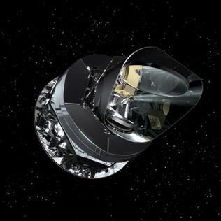
Figure: Artist’s impression of the Planck spacecraft which measured the Cosmic Microwave Background between 2009 and 2013.
The objective of the Planck spacecraft was to measure the anisotropy and statistics of the Cosmic Microwave Background. This was important, because if the standard model of the Universe is correct the variations around the very high temperature of the Universe of the CMB should be distributed according to a Gaussian process.3 Currently our best estimates show this to be the case (Elsner et al., 2016, 2015; Jaffe et al., 1998; Pontzen and Peiris, 2010).
To the high degree of precision that we could measure with the Planck space telescope, the CMB appears to be a Gaussian process. The parameters of its covariance function are given by the fundamental parameters of the universe, for example the amount of dark matter and matter in the universe
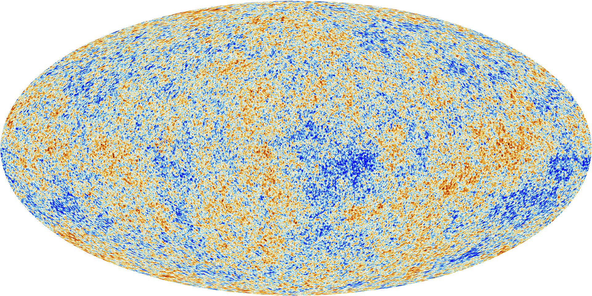
Figure: The cosmic microwave background is, to a very high degree of precision, a Gaussian process. The parameters of its covariance function are given by fundamental parameters of the universe, such as the amount of dark matter and mass.
Simulating a CMB Map
The simulation was created by Boris Leistedt, see the original Jupyter notebook here.
Here we use that code to simulate our own universe and sample from what it looks like.
First, we install some specialist software as well as matplotlib, scipy, numpy we require
%pip install camb%pip install healpyimport healpy as hp
import camb
from camb import model, initialpowerNow we use the theoretical power spectrum to design the covariance function.
nside = 512  # Healpix parameter, giving 12*nside**2 equal-area pixels on the sphere.
lmax = 3*nside # band-limit. Should be 2*nside < lmax < 4*nside to get information content.
Now we design our Universe. It is parameterized according to the \(\Lambda\)CDM model. The variables are as follows. H0 is the Hubble parameter (in Km/s/Mpc). The ombh2 is Physical Baryon density parameter. The omch2 is the physical dark matter density parameter. mnu is the sum of the neutrino masses (in electron Volts). omk is the \(\Omega_k\) is the curvature parameter, which is here set to 0, giving the minimal six parameter Lambda-CDM model. tau is the reionization optical depth.
Then we set ns, the “scalar spectral index.” This was estimated by Planck to be 0.96. Then there’s r, the ratio of the tensor power spectrum to scalar power spectrum. This has been estimated by Planck to be under 0.11. Here we set it to zero. These parameters are associated with inflation.
# Mostly following http://camb.readthedocs.io/en/latest/CAMBdemo.html with parameters from https://en.wikipedia.org/wiki/Lambda-CDM_model

pars = camb.CAMBparams()
pars.set_cosmology(H0=67.74, ombh2=0.0223, omch2=0.1188, mnu=0.06, omk=0, tau=0.066)
pars.InitPower.set_params(ns=0.96, r=0)
Having set the parameters, we now use the python software “Code for Anisotropies in the Microwave Background” to get the results.
pars.set_for_lmax(lmax, lens_potential_accuracy=0);
results = camb.get_results(pars)
powers = results.get_cmb_power_spectra(pars)
totCL = powers['total']
unlensedCL = powers['unlensed_scalar']

ells = np.arange(totCL.shape[0])
Dells = totCL[:, 0]
Cells = Dells * 2*np.pi / ells / (ells + 1)  # change of convention to get C_ell
Cells[0:2] = 0
cmbmap = hp.synfast(Cells, nside,
lmax=lmax, mmax=None, alm=False, pol=False,
pixwin=False, fwhm=0.0, sigma=None, new=False, verbose=True)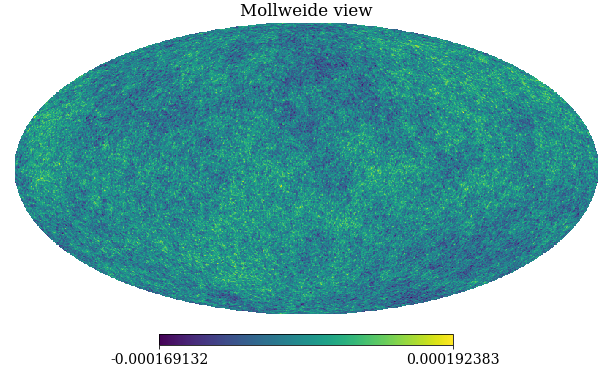
Figure: A simulation of the Cosmic Microwave Background obtained through sampling from the relevant Gaussian process covariance (in polar co-ordinates).
The world we see today, of course, is not a Gaussian process. There are many discontinuities, for example, in the density of matter, and therefore in the temperature of the Universe.
 \(=f\Bigg(\)\(\Bigg)\)
Figure: What we observe today is some non-linear function of the cosmic microwave background.
We can think of today’s observed Universe, though, as a being a consequence of those temperature fluctuations in the CMB. Those fluctuations are only order \(10^{-6}\) of the scale of the overall temperature of the Universe. But minor fluctuations in that density are what triggered the pattern of formation of the Galaxies. They determined how stars formed and created the elements that are the building blocks of our Earth (Vogelsberger et al., 2020).
Modern Review
A Unifying Framework for Gaussian Process Pseudo-Point Approximations using Power Expectation Propagation Bui et al. (2017)
Deep Gaussian Processes and Variational Propagation of Uncertainty Damianou (2015)
%pip install gpyGPy: A Gaussian Process Framework in Python
Gaussian processes are a flexible tool for non-parametric analysis with uncertainty. The GPy software was started in Sheffield to provide a easy to use interface to GPs. One which allowed the user to focus on the modelling rather than the mathematics.

Figure: GPy is a BSD licensed software code base for implementing Gaussian process models in Python. It is designed for teaching and modelling. We welcome contributions which can be made through the GitHub repository https://github.com/SheffieldML/GPy
GPy is a BSD licensed software code base for implementing Gaussian process models in python. This allows GPs to be combined with a wide variety of software libraries.
The software itself is available on GitHub and the team welcomes contributions.
The aim for GPy is to be a probabilistic-style programming language, i.e., you specify the model rather than the algorithm. As well as a large range of covariance functions the software allows for non-Gaussian likelihoods, multivariate outputs, dimensionality reduction and approximations for larger data sets.
The documentation for GPy can be found here.
This notebook depends on PyDeepGP. This library can be installed via pip.
%pip install --upgrade git+https://github.com/SheffieldML/PyDeepGP.git# Late bind setup methods to DeepGP object
from mlai.deepgp_tutorial import initialize
from mlai.deepgp_tutorial import staged_optimize
from mlai.deepgp_tutorial import posterior_sample
from mlai.deepgp_tutorial import visualize
from mlai.deepgp_tutorial import visualize_pinball
import deepgp
deepgp.DeepGP.initialize=initialize
deepgp.DeepGP.staged_optimize=staged_optimize
deepgp.DeepGP.posterior_sample=posterior_sample
deepgp.DeepGP.visualize=visualize
deepgp.DeepGP.visualize_pinball=visualize_pinballOlympic Marathon Data
|
|
The first thing we will do is load a standard data set for regression modelling. The data consists of the pace of Olympic Gold Medal Marathon winners for the Olympics from 1896 to present. Let’s load in the data and plot.
%pip install podsimport numpy as np
import podsdata = pods.datasets.olympic_marathon_men()
x = data['X']
y = data['Y']
offset = y.mean()
scale = np.sqrt(y.var())
yhat = (y - offset)/scaleFigure: Olympic marathon pace times since 1896.
Things to notice about the data include the outlier in 1904, in that year the Olympics was in St Louis, USA. Organizational problems and challenges with dust kicked up by the cars following the race meant that participants got lost, and only very few participants completed. More recent years see more consistently quick marathons.
Alan Turing
|
|
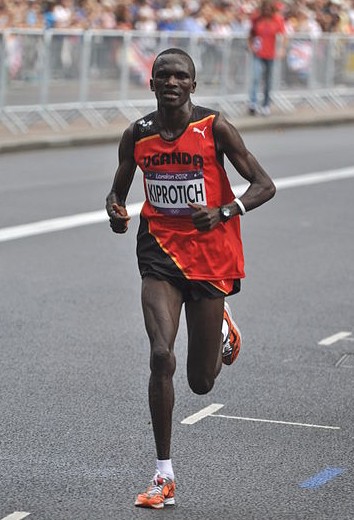
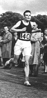
Figure: Alan Turing, in 1946 he was only 11 minutes slower than the winner of the 1948 games. Would he have won a hypothetical games held in 1946? Source: Alan Turing Internet Scrapbook.
If we had to summarise the objectives of machine learning in one word, a very good candidate for that word would be generalization. What is generalization? From a human perspective it might be summarised as the ability to take lessons learned in one domain and apply them to another domain. If we accept the definition given in the first session for machine learning, \[ \text{data} + \text{model} \stackrel{\text{compute}}{\rightarrow} \text{prediction} \] then we see that without a model we can’t generalise: we only have data. Data is fine for answering very specific questions, like “Who won the Olympic Marathon in 2012?” because we have that answer stored, however, we are not given the answer to many other questions. For example, Alan Turing was a formidable marathon runner, in 1946 he ran a time 2 hours 46 minutes (just under four minutes per kilometer, faster than I and most of the other Endcliffe Park Run runners can do 5 km). What is the probability he would have won an Olympics if one had been held in 1946?
To answer this question we need to generalize, but before we formalize the concept of generalization let’s introduce some formal representation of what it means to generalize in machine learning.
Gaussian Process Fit
Our first objective will be to perform a Gaussian process fit to the data, we’ll do this using the GPy software.
import GPym_full = GPy.models.GPRegression(x,yhat)
_ = m_full.optimize() # Optimize parameters of covariance functionThe first command sets up the model, then m_full.optimize() optimizes the parameters of the covariance function and the noise level of the model. Once the fit is complete, we’ll try creating some test points, and computing the output of the GP model in terms of the mean and standard deviation of the posterior functions between 1870 and 2030. We plot the mean function and the standard deviation at 200 locations. We can obtain the predictions using y_mean, y_var = m_full.predict(xt)
xt = np.linspace(1870,2030,200)[:,np.newaxis]
yt_mean, yt_var = m_full.predict(xt)
yt_sd=np.sqrt(yt_var)Now we plot the results using the helper function in mlai.plot.
Figure: Gaussian process fit to the Olympic Marathon data. The error bars are too large, perhaps due to the outlier from 1904.
Fit Quality
In the fit we see that the error bars (coming mainly from the noise variance) are quite large. This is likely due to the outlier point in 1904, ignoring that point we can see that a tighter fit is obtained. To see this make a version of the model, m_clean, where that point is removed.
x_clean=np.vstack((x[0:2, :], x[3:, :]))
y_clean=np.vstack((yhat[0:2, :], yhat[3:, :]))
m_clean = GPy.models.GPRegression(x_clean,y_clean)
_ = m_clean.optimize()Deep GP Fit
Let’s see if a deep Gaussian process can help here. We will construct a deep Gaussian process with one hidden layer (i.e. one Gaussian process feeding into another).
Build a Deep GP with an additional hidden layer (one dimensional) to fit the model.
import GPy
import deepgphidden = 1
m = deepgp.DeepGP([y.shape[1],hidden,x.shape[1]],Y=yhat, X=x, inits=['PCA','PCA'],
kernels=[GPy.kern.RBF(hidden,ARD=True),
GPy.kern.RBF(x.shape[1],ARD=True)], # the kernels for each layer
num_inducing=50, back_constraint=False)# Call the initalization
m.initialize()Now optimize the model.
for layer in m.layers:
layer.likelihood.variance.constrain_positive(warning=False)
m.optimize(messages=True,max_iters=10000)m.staged_optimize(messages=(True,True,True))Olympic Marathon Data Deep GP
Figure: Deep GP fit to the Olympic marathon data. Error bars now change as the prediction evolves.
Olympic Marathon Data Deep GP
Figure: Point samples run through the deep Gaussian process show the distribution of output locations.
Fitted GP for each layer
Now we explore the GPs the model has used to fit each layer. First of all, we look at the hidden layer.
Figure: The mapping from input to the latent layer is broadly, with some flattening as time goes on. Variance is high across the input range.
Figure: The mapping from the latent layer to the output layer.
Olympic Marathon Pinball Plot
Figure: A pinball plot shows the movement of the ‘ball’ as it passes through each layer of the Gaussian processes. Mean directions of movement are shown by lines. Shading gives one standard deviation of movement position. At each layer, the uncertainty is reset. The overal uncertainty is the cumulative uncertainty from all the layers. There is some grouping of later points towards the right in the first layer, which also injects a large amount of uncertainty. Due to flattening of the curve in the second layer towards the right the uncertainty is reduced in final output.
The pinball plot shows the flow of any input ball through the deep Gaussian process. In a pinball plot a series of vertical parallel lines would indicate a purely linear function. For the olypmic marathon data we can see the first layer begins to shift from input towards the right. Note it also does so with some uncertainty (indicated by the shaded backgrounds). The second layer has less uncertainty, but bunches the inputs more strongly to the right. This input layer of uncertainty, followed by a layer that pushes inputs to the right is what gives the heteroschedastic noise.
Step Function
Next we consider a simple step function data set.
num_low=25
num_high=25
gap = -.1
noise=0.0001
x = np.vstack((np.linspace(-1, -gap/2.0, num_low)[:, np.newaxis],
np.linspace(gap/2.0, 1, num_high)[:, np.newaxis]))
y = np.vstack((np.zeros((num_low, 1)), np.ones((num_high,1))))
scale = np.sqrt(y.var())
offset = y.mean()
yhat = (y-offset)/scaleStep Function Data
Figure: Simulation study of step function data artificially generated. Here there is a small overlap between the two lines.
Step Function Data GP
We can fit a Gaussian process to the step function data using GPy as follows.
m_full = GPy.models.GPRegression(x,yhat)
_ = m_full.optimize() # Optimize parameters of covariance functionWhere GPy.models.GPRegression() gives us a standard GP regression model with exponentiated quadratic covariance function.
The model is optimized using m_full.optimize() which calls an L-BGFS gradient based solver in python.
Figure: Gaussian process fit to the step function data. Note the large error bars and the over-smoothing of the discontinuity. Error bars are shown at two standard deviations.
The resulting fit to the step function data shows some challenges. In particular, the over smoothing at the discontinuity. If we know how many discontinuities there are, we can parameterize them in the step function. But by doing this, we form a semi-parametric model. The parameters indicate how many discontinuities are, and where they are. They can be optimized as part of the model fit. But if new, unforeseen, discontinuities arise when the model is being deployed in practice, these won’t be accounted for in the predictions.
Step Function Data Deep GP
First we initialize a deep Gaussian process with three latent layers (four layers total). Within each layer we create a GP with an exponentiated quadratic covariance (GPy.kern.RBF).
At each layer we use 20 inducing points for the variational approximation.
layers = [y.shape[1], 1, 1, 1,x.shape[1]]
inits = ['PCA']*(len(layers)-1)
kernels = []
for i in layers[1:]:
kernels += [GPy.kern.RBF(i)]
m = deepgp.DeepGP(layers,Y=yhat, X=x,
inits=inits,
kernels=kernels, # the kernels for each layer
num_inducing=20, back_constraint=False)Once the model is constructed we initialize the parameters, and perform the staged optimization which starts by optimizing variational parameters with a low noise and proceeds to optimize the whole model.
m.initialize()
m.staged_optimize()We plot the output of the deep Gaussian process fitted to the step data as follows.
The deep Gaussian process does a much better job of fitting the data. It handles the discontinuity easily, and error bars drop to smaller values in the regions of data.
Figure: Deep Gaussian process fit to the step function data.
Step Function Data Deep GP
The samples of the model can be plotted with the helper function from mlai.plot, model_sample
The samples from the model show that the error bars, which are informative for Gaussian outputs, are less informative for this model. They make clear that the data points lie, in output mainly at 0 or 1, or occasionally in between.
Figure: Samples from the deep Gaussian process model for the step function fit.
The visualize code allows us to inspect the intermediate layers in the deep GP model to understand how it has reconstructed the step function.
Figure: From top to bottom, the Gaussian process mapping function that makes up each layer of the resulting deep Gaussian process.
A pinball plot can be created for the resulting model to understand how the input is being translated to the output across the different layers.
Figure: Pinball plot of the deep GP fitted to the step function data. Each layer of the model pushes the ‘ball’ towards the left or right, saturating at 1 and 0. This causes the final density to be be peaked at 0 and 1. Transitions occur driven by the uncertainty of the mapping in each layer.
import podsdata = pods.datasets.mcycle()
x = data['X']
y = data['Y']
scale=np.sqrt(y.var())
offset=y.mean()
yhat = (y - offset)/scaleMotorcycle Helmet Data
Figure: Motorcycle helmet data. The data consists of acceleration readings on a motorcycle helmet undergoing a collision. The data exhibits heteroschedastic (time varying) noise levles and non-stationarity.
m_full = GPy.models.GPRegression(x,yhat)
_ = m_full.optimize() # Optimize parameters of covariance functionMotorcycle Helmet Data GP
Figure: Gaussian process fit to the motorcycle helmet accelerometer data.
Motorcycle Helmet Data Deep GP
import deepgplayers = [y.shape[1], 1, x.shape[1]]
inits = ['PCA']*(len(layers)-1)
kernels = []
for i in layers[1:]:
kernels += [GPy.kern.RBF(i)]
m = deepgp.DeepGP(layers,Y=yhat, X=x,
inits=inits,
kernels=kernels, # the kernels for each layer
num_inducing=20, back_constraint=False)
m.initialize()m.staged_optimize(iters=(1000,1000,10000), messages=(True, True, True))Figure: Deep Gaussian process fit to the motorcycle helmet accelerometer data.
Motorcycle Helmet Data Deep GP
Figure: Samples from the deep Gaussian process as fitted to the motorcycle helmet accelerometer data.
Motorcycle Helmet Data Latent 1
Figure: Mappings from the input to the latent layer for the motorcycle helmet accelerometer data.
Motorcycle Helmet Data Latent 2
Figure: Mappings from the latent layer to the output layer for the motorcycle helmet accelerometer data.
Motorcycle Helmet Pinball Plot
Figure: Pinball plot for the mapping from input to output layer for the motorcycle helmet accelerometer data.
Subsample of the MNIST Data
We will look at a sub-sample of the MNIST digit data set.
First load in the MNIST data set from scikit learn. This can take a little while because it’s large to download.
from sklearn.datasets import fetch_openmlmnist = fetch_openml('mnist_784')Sub-sample the dataset to make the training faster.
import numpy as npnp.random.seed(0)
digits = [0,1,2,3,4]
N_per_digit = 100
Y = []
labels = []
for d in digits:
imgs = mnist['data'][mnist['target']==str(d)]
Y.append(imgs.loc[np.random.permutation(imgs.index)[:N_per_digit]])
labels.append(np.ones(N_per_digit)*d)
Y = np.vstack(Y).astype(np.float64)
labels = np.hstack(labels)
Y /= 255Fitting a Deep GP to a the MNIST Digits Subsample
We now look at the deep Gaussian processes’ capacity to perform unsupervised learning.
Fit a Deep GP
We’re going to fit a Deep Gaussian process model to the MNIST data with two hidden layers. Each of the two Gaussian processes (one from the first hidden layer to the second, one from the second hidden layer to the data) has an exponentiated quadratic covariance.
import deepgp
import GPynum_latent = 2
num_hidden_2 = 5
m = deepgp.DeepGP([Y.shape[1],num_hidden_2,num_latent],
Y,
kernels=[GPy.kern.RBF(num_hidden_2,ARD=True),
GPy.kern.RBF(num_latent,ARD=False)],
num_inducing=50, back_constraint=False,
encoder_dims=[[200],[200]])Initialization
Just like deep neural networks, there are some tricks to intitializing these models. The tricks we use here include some early training of the model with model parameters constrained. This gives the variational inducing parameters some scope to tighten the bound for the case where the noise variance is small and the variances of the Gaussian processes are around 1.
m.obslayer.likelihood.variance[:] = Y.var()*0.01
for layer in m.layers:
layer.kern.variance.fix(warning=False)
layer.likelihood.variance.fix(warning=False)We now we optimize for a hundred iterations with the constrained model.
m.optimize(messages=False,max_iters=100)Now we remove the fixed constraint on the kernel variance parameters, but keep the noise output constrained, and run for a further 100 iterations.
for layer in m.layers:
layer.kern.variance.constrain_positive(warning=False)
m.optimize(messages=False,max_iters=100)Finally we unconstrain the layer likelihoods and allow the full model to be trained for 1000 iterations.
for layer in m.layers:
    layer.likelihood.variance.constrain_positive(warning=False)
m.optimize(messages=True,max_iters=10000)Visualize the latent space of the top layer
Now the model is trained, let’s plot the mean of the posterior distributions in the top latent layer of the model.
Figure: Latent space for the deep Gaussian process learned through unsupervised learning and fitted to a subset of the MNIST digits subsample.
Visualize the latent space of the intermediate layer
We can also visualize dimensions of the intermediate layer. First the lengthscale of those dimensions is given by
m.obslayer.kern.lengthscaleGenerate From Model
Now we can take a look at a sample from the model, by drawing a Gaussian random sample in the latent space and propagating it through the model.
rows = 10
cols = 20
t=np.linspace(-1, 1, rows*cols)[:, None]
kern = GPy.kern.RBF(1,lengthscale=0.05)
cov = kern.K(t, t)
x = np.random.multivariate_normal(np.zeros(rows*cols), cov, num_latent).T
Figure: These digits are produced by taking a tour of the two dimensional latent space (as described by a Gaussian process sample) and mapping the tour into the data space. We visualize the mean of the mapping in the images.
Deep NNs as Point Estimates for Deep GPs
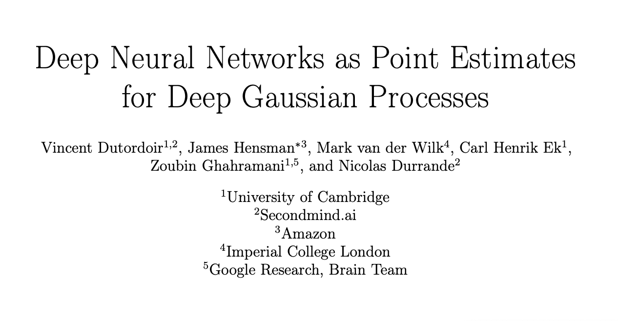
Figure: Deep Neural Networks as Point Estimates for Deep Gaussian Processes by Dutordoir et al. (2021) shows how deep neural networks can represent the mean function of an approximate deep GP.
A very promising idea was recently presented by Dutordoir et al. (2021). They note that the ReLU activiation functions we use in the neural network can be seen as the consequence of a basis function defined on a circle (or a hypersphere in higher dimensions) being projected onto the real line (or hyperplane) as show in Figure . This allows them to construct a covariance function on the hypersphere that is stationary.
ReLU as a Spherical Basis
Figure: The rectified linear unit can be seen as a basis function that lives on a spherical domain being projected onto the real line.
Figure: The soft ReLU can also be seen as a basis function that lives on a spherical domain being projected onto the real line.
Spherical Harmonics
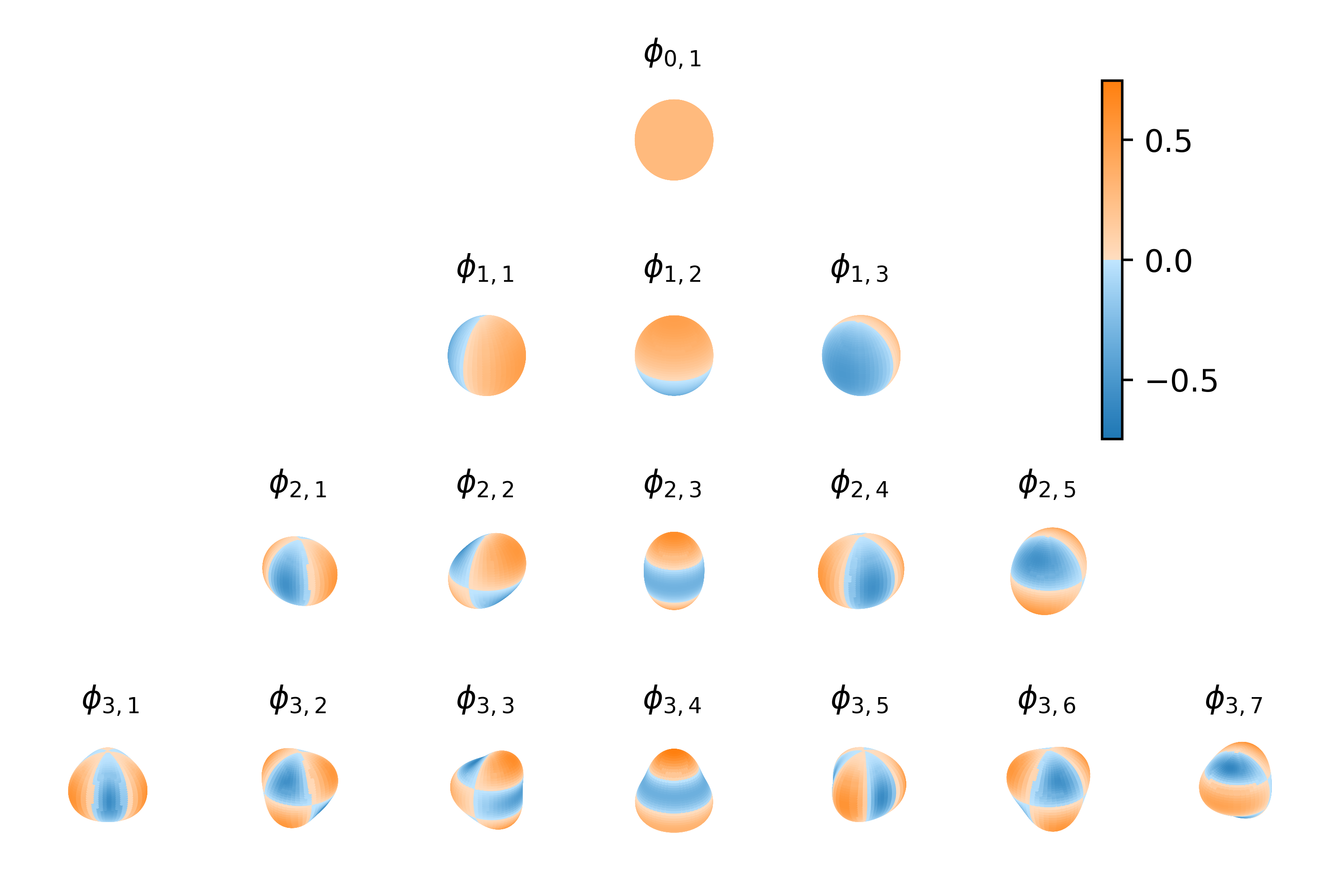
Figure: The method exploits interdomain inducing variables, reinterpreting the ReLU covariance function as a stationary covariance on the spherical domain that has been projected to the real line.
Applying variational inference techniques to the resulting model (see e.g. Hensman et al. (n.d.),Hensman and Lawrence (2014)) and making use of interdomain variational approximations (Lázaro-Gredilla et al. (2010),Álvarez et al. (2010),Hensman et al. (2018)) causes the mean function approximation of the Gaussian process to have the same form as a fully connected deep neural network. This inspires the idea to use a trained neural network to initialise the deep Gaussian process.
Predictions on Banana Data
Figure: The banana data is an artificially sampled data set with two classes (from Rätsch et al. (2001)).
Figure: One layer deep GP fit showing the neural network point estimate (from Dutordoir et al. (2021)).
Figure: One layer deep GP fit showing the activated deep Gaussian process fit (from Dutordoir et al. (2021)).
The results of doing this on the banana data (Figure Rätsch et al. (2001)) can be seen with the neural network solution in Figure and the neural network activated deep GP solution given in Figure .
Deep Health
Figure: The deep health model uses different layers of abstraction in the deep Gaussian process to represent information about diagnostics and treatment to model interelationships between a patients different data modalities.
From a machine learning perspective, we’d like to be able to interrelate all the different modalities that are informative about the state of the disease. For deep health, the notion is that the state of the disease is appearing at the more abstract levels, as we descend the model, we express relationships between the more abstract concept, that sits within the physician’s mind, and the data we can measure.
Thanks!
For more information on these subjects and more you might want to check the following resources.
- twitter: @lawrennd
- podcast: The Talking Machines
- newspaper: Guardian Profile Page
- blog: http://inverseprobability.com
References
The logarithm of a number less than one is negative, for a number greater than one the logarithm is positive. So if odds are greater than evens (odds-on) the log-odds are positive, if the odds are less than evens (odds-against) the log-odds will be negative.↩︎
The NTSB Report on the accident can be found online here: https://www.ntsb.gov/investigations/Pages/HWY18FH010.aspx.↩︎
Most of my understanding of this is taken from conversations with Kyle Cranmer, a physicist who makes extensive use of machine learning methods in his work. See e.g. Mishra-Sharma and Cranmer (2020) from Kyle and Siddharth Mishra-Sharma. Of course, any errors in the above text are mine and do not stem from Kyle.↩︎