Abstract

In this session we introduce the notion of emulation and systems modeling with Gaussian processes.

We may regard the present state of the universe as the effect of its past and the cause of its future. An intellect which at a certain moment would know all forces that set nature in motion, and all positions of all items of which nature is composed, …

… if this intellect were also vast enough to submit these data to analysis, it would embrace in a single formula the movements of the greatest bodies of the universe and those of the tiniest atom; for such an intellect nothing would be uncertain and the future just like the past would be present before its eyes.

— Pierre Simon Laplace (Laplace, 1814)

Game of Life

John Horton Conway was a mathematician who developed a game known as the Game of Life. He died in April 2020, but since he invented the game, he was in effect ‘god’ for this game. But as we will see, just inventing the rules doesn’t give you omniscience in the game.

The Game of Life is played on a grid of squares, or pixels. Each pixel is either on or off. The game has no players, but a set of simple rules that are followed at each turn the rules are.

Life Rules

John Conway’s game of life is a cellular automata where the cells obey three very simple rules. The cells live on a rectangular grid, so that each cell has 8 possible neighbors.

loneliness

Figure: ‘Death’ through loneliness in Conway’s game of life. If a cell is surrounded by less than three cells, it ‘dies’ through loneliness.

The game proceeds in turns, and at each location in the grid is either alive or dead. Each turn, a cell counts its neighbors. If there are two or fewer neighbors, the cell ‘dies’ of ‘loneliness.’

overcrowding

Figure: ‘Death’ through overpopulation in Conway’s game of life. If a cell is surrounded by more than three cells, it ‘dies’ through loneliness.

If there are four or more neigbors, the cell ‘dies’ from ‘overcrowding.’ If there are three neigbors, the cell persists, or if it is currently dead, a new cell is born.

birth

Figure: Birth in Conway’s life. Any position surounded by precisely three live cells will give birth to a new cell at the next turn.

And that’s it. Those are the simple ‘physical laws’ for Conway’s game.

The game leads to patterns emerging, some of these patterns are static, but some oscillate in place, with varying periods. Others oscillate, but when they complete their cycle they’ve translated to a new location, in other words they move. In Life the former are known as oscillators and the latter as spaceships.

Loafers and Gliders

John Horton Conway, as the creator of the game of life, could be seen somehow as the god of this small universe. He created the rules. The rules are so simple that in many senses he, and we, are all-knowing in this space. But despite our knowledge, this world can still ‘surprise’ us. From the simple rules, emergent patterns of behaviour arise. These include static patterns that don’t change from one turn to the next. They also include, oscillators, that pulse between different forms across different periods of time. A particular form of oscillator is known as a ‘spaceship,’ this is one that moves across the board as the game evolves. One of the simplest and earliest spaceships to be discovered is known as the glider.

Glider (1969)

Figure: Left A Glider pattern discovered 1969 by Richard K. Guy. Right. John Horton Conway, creator of Life (1937-2020). The glider is an oscillator that moves diagonally after creation. From the simple rules of Life it’s not obvious that such an object does exist, until you do the necessary computation.

The glider was ‘discovered’ in 1969 by Richard K. Guy. What do we mean by discovered in this context? Well, as soon as the game of life is defined, objects such as the glider do somehow exist, but the many configurations of the game mean that it takes some time for us to see one and know it exists. This means, that despite being the creator, Conway, and despite the rules of the game being simple, and despite the rules being deterministic, we are not ‘omniscient’ in any simplistic sense. It requires computation to ‘discover’ what can exist in this universe once it’s been defined.

Figure: The Gosper glider gun is a configuration that creates gliders. A new glider is released after every 30 turns.

These patterns had to be discovered, in the same way that a scientist might discover a disease, or an explorer a new land. For example, the Gosper glider gun was discovered by Bill Gosper in 1970. It is a pattern that creates a new glider every 30 turns of the game.

Despite widespread interest in Life, some of its patterns were only very recently discovered like the Loafer, discovered in 2013 by Josh Ball. So despite the game having existed for over forty years, and the rules of the game being simple, there are emergent behaviours that are unknown.

Loafer (2013)

Figure: Left A Loafer pattern discovered by Josh Ball in 2013. Right. John Horton Conway, creator of Life (1937-2020).

Once these patterns are discovered, they are combined (or engineered) to create new Life patterns that do some remarkable things. For example, there’s a life pattern that runs a Turing machine, or more remarkably there’s a Life pattern that runs Life itself.

Figure: The Game of Life running in Life. The video is drawing out recursively showing pixels that are being formed by filling cells with moving spaceships. Each individual pixel in this game of life is made up of \(2048 \times 2048\) pixels called an OTCA metapixel.

To find out more about the Game of Life you can watch this video by Alan Zucconi or read his associated blog post.

Figure: An introduction to the Game of Life by Alan Zucconi.

Contrast this with our situation where in ‘real life’ we don’t know the simple rules of the game, the state space is larger, and emergent behaviors (hurricanes, earthquakes, volcanos, climate change) have direct consequences for our daily lives, and we understand why the process of ‘understanding’ the physical world is so difficult. We also see immediately how much easier we might expect the physical sciences to be than the social sciences, where the emergent behaviors are contingent on highly complex human interactions.

We summarize this notion as \[ \text{data} + \text{model} \stackrel{\text{compute}}{\rightarrow} \text{prediction} \] As we pointed out, there is an irony in Laplace’s demon forming the cornerstone of a movement known as ‘determinism,’ because Laplace wrote about this idea in an essay on probabilities. The more important quote in the essay was

Laplace’s Gremlin

The curve described by a simple molecule of air or vapor is regulated in a manner just as certain as the planetary orbits; the only difference between them is that which comes from our ignorance. Probability is relative, in part to this ignorance, in part to our knowledge. We know that of three or greater number of events a single one ought to occur; but nothing induces us to believe that one of them will occur rather than the others. In this state of indecision it is impossible for us to announce their occurrence with certainty. It is, however, probable that one of these events, chosen at will, will not occur because we see several cases equally possible which exclude its occurrence, while only a single one favors it.

— Pierre-Simon Laplace (Laplace, 1814), pg 5

The representation of ignorance through probability is the true message of Laplace, I refer to this message as “Laplace’s gremlin,” because it is the gremlin of uncertainty that interferes with the demon of determinism to mean that our predictions are not deterministic.

Our separation of the uncertainty into the data, the model and the computation give us three domains in which our doubts can creep into our ability to predict. Over the last three lectures we’ve introduced some of the basic tools we can use to unpick this uncertainty. You’ve been introduced to, (or have yow reviewed) Bayes’ rule. The rule, which is a simple consequence of the product rule of probability, is the foundation of how we update our beliefs in the presence of new information.

The real point of Laplace’s essay was that we don’t have access to all the data, we don’t have access to a complete physical understanding, and as the example of the Game of Life shows, even if we did have access to both (as we do for “Conway’s universe”) we still don’t have access to all the compute that we need to make deterministic predictions. There is uncertainty in the system which means we can’t make precise predictions.

I like to call this “Laplace’s Gremlin.” Gremlins are imaginary creatures used as an explanation of failure in aircraft, causing crashes. In that sense the Gremlin represents the uncertainty that a pilot felt about what might go wrong in a plane which might be “theoretically sound” but in practice is poorly maintained or exposed to conditions that take it beyond its design criteria. Laplace’s gremlin is all the things that your model, data and ability to compute don’t account for bringing about failures in your ability to predict. Laplace’s Gremlin is the uncertainty in the system.

Figure: Gremlins are seen as the cause of a number of challenges in this World War II poster.

Simulation System

An example of a complex decision-making system might be a climate model, in such a system there are separate models for the atmosphere, the ocean and the land.

The components of these systems include flowing of currents, chemical interactions in the upper atmosphere, evaporation of water etc..

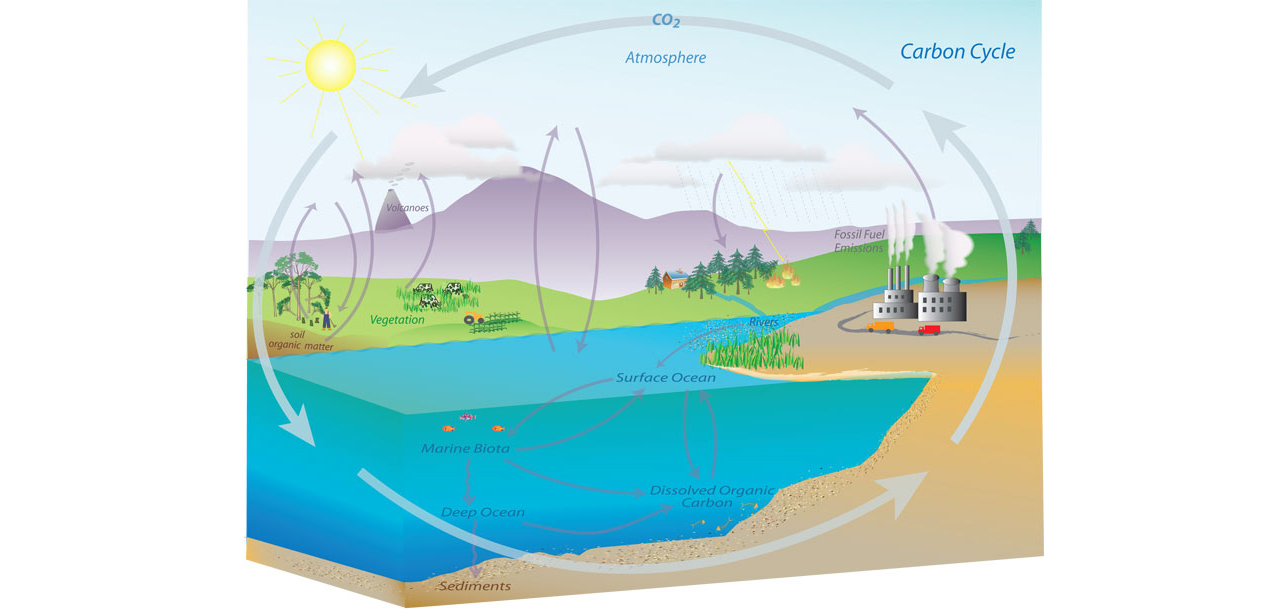
Figure: Representation of the Carbon Cycle from the US National Oceanic and Atmospheric Administration. While everything is interconnected in the system, we can decompose into separate models for atmosphere, ocean, land.

The influence of human activity also needs to be incorporated and modelled so we can make judgments about how to mitigate the effects of global warming.

Figure: The components of a simulation system for climate modelling.

Monolithic System

The classical approach to building these systems was a ‘monolithic system.’ Built in a similar way to the successful applications software such as Excel or Word, or large operating systems, a single code base was constructed. The complexity of such code bases run to many lines.

In practice, shared dynamically linked libraries may be used for aspects such as user interface, or networking, but the software often has many millions of lines of code. For example, the Microsoft Office suite is said to contain over 30 million lines of code.

Figure: A potential path of models in a machine learning system.

Service Oriented Architecture

Such software is not only difficult to develop, but also to scale when computation demands increase. For example, Amazon’s original website software (called Obidos) was a monolithic design but by the early noughties it was becoming difficult to sustain and maintain. The software was phased out in 2006 to be replaced by a modularized software known as a ‘service-oriented architecture.’

In Service Oriented Architecture, or “Software as a Service” the idea is that code bases are modularized and communicate with one another using network requests. A standard approach is to use a REST API. So, rather than a single monolithic code base, the code is developed with individual services that handle the different requests.

The simulation software is turned inside out to expose the individual components to the operator.

Figure: A potential path of models in a machine learning system.

This is the landscape we now find ourselves in for software development. In practice, each of these services is often ‘owned’ and maintained by an individual team. The team is judged by the quality of their service provision. They work to detailed specifications on what their service should output, what its availability should be and other objectives like speed of response. This allows for conditional independence between teams and for faster development.

One question is to what extent is the same approach possible/desirable for scientific models? The components we listed above are already separated and often run independently. But those components themselves are made up of other sub-components that could also be exposed in a similar manner to software-as-a-service, giving us the notion of “simulation as a service.”

One thing about working in an industrial environment, is the way that short-term thinking actions become important. For example, in Formula One, the teams are working on a two-week cycle to digest information from the previous week’s race and incorporate updates to the car or their strategy.

However, businesses must also think about more medium-term horizons. For example, in Formula 1 you need to worry about next year’s car. So while you’re working on updating this year’s car, you also need to think about what will happen for next year and prioritize these conflicting needs appropriately.

In the Amazon supply chain, there are the equivalent demands. If we accept that an artificial intelligence is just an automated decision-making system. And if we measure in terms of money automatically spent, or goods automatically moved, then Amazon’s buying system is perhaps the world’s largest AI.

Those decisions are being made on short time schedules; purchases are made by the system on weekly cycles. But just as in Formula 1, there is also a need to think about what needs to be done next month, next quarter and next year. Planning meetings are held not only on a weekly basis (known as weekly business reviews), but monthly, quarterly, and then yearly meetings for planning spends and investments.

Amazon is known for being longer term thinking than many companies, and a lot of this is coming from the CEO. One quote from Jeff Bezos that stuck with me was the following.

“I very frequently get the question: ‘What’s going to change in the next 10 years?’ And that is a very interesting question; it’s a very common one. I almost never get the question: ‘What’s not going to change in the next 10 years?’ And I submit to you that that second question is actually the more important of the two – because you can build a business strategy around the things that are stable in time. … [I]n our retail business, we know that customers want low prices, and I know that’s going to be true 10 years from now. They want fast delivery; they want vast selection. It’s impossible to imagine a future 10 years from now where a customer comes up and says, ‘Jeff I love Amazon; I just wish the prices were a little higher,’ [or] ‘I love Amazon; I just wish you’d deliver a little more slowly.’ Impossible. And so the effort we put into those things, spinning those things up, we know the energy we put into it today will still be paying off dividends for our customers 10 years from now. When you have something that you know is true, even over the long term, you can afford to put a lot of energy into it.”

This quote is incredibly important for long term thinking. Indeed, it’s a failure of many of our simulations that they focus on what is going to happen, not what will not happen. In Amazon, this meant that there was constant focus on these three areas, keeping costs low, making delivery fast and improving selection. For example, shortly before I left Amazon moved its entire US network from two-day delivery to one-day delivery. This involves changing the way the entire buying system operates. Or, more recently, the company has had to radically change the portfolio of products it buys in the face of Covid19.

Figure: Experiment, analyze and design is a flywheel of knowledge that is the dual of the model, data and compute. By running through this spiral, we refine our hypothesis/model and develop new experiments which can be analyzed to further refine our hypothesis.

From the perspective of the team that we had in the supply chain, we looked at what we most needed to focus on. Amazon moves very quickly, but we could also take a leaf out of Jeff’s book, and instead of worrying about what was going to change, remember what wasn’t going to change.

We don’t know what science we’ll want to do in five years’ time, but we won’t want slower experiments, we won’t want more expensive experiments and we won’t want a narrower selection of experiments.

As a result, our focus was on how to speed up the process of experiments, increase the diversity of experiments that we can do, and keep the experiments price as low as possible.

The faster the innovation flywheel can be iterated, then the quicker we can ask about different parts of the supply chain, and the better we can tailor systems to answering those questions.

We need faster, cheaper and more diverse experiments which implies we need better ecosystems for experimentation. This has led us to focus on the software frameworks we’re using to develop machine learning systems including data oriented architectures (Borchert (2020);(Lawrence-doa19?);Vorhemus and Schikuta (2017);Joshi (2007)), data maturity assessments (Lawrence et al. (2020)) and data readiness levels (See this blog post on Data Readiness Levels. and Lawrence (2017);The DELVE Initiative (2020))

Statistical Emulation

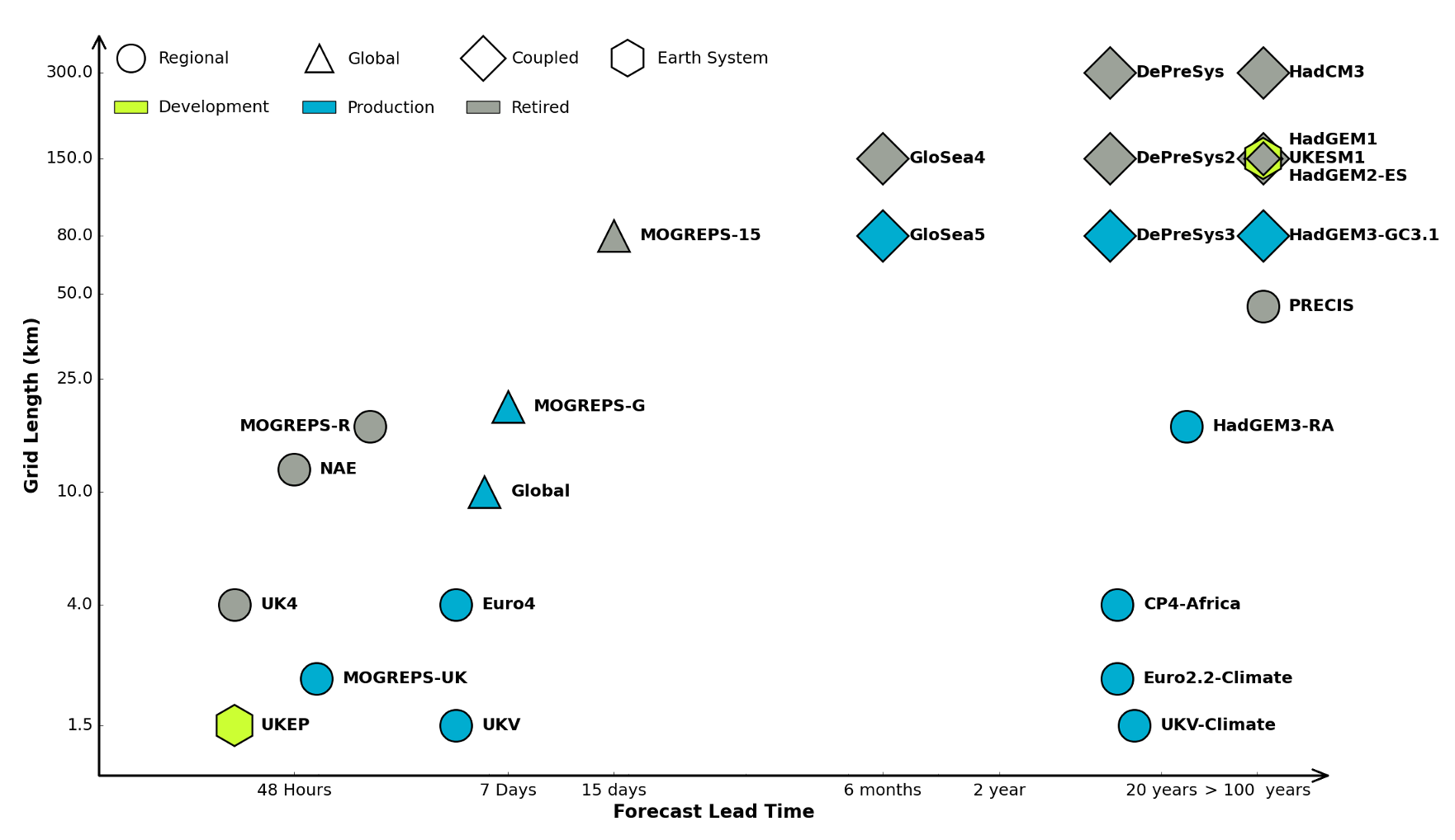
Figure: The UK Met office runs a shared code base for its simulations of climate and the weather. This plot shows the different spatial and temporal scales used.

In many real-world systems, decisions are made through simulating the environment. Simulations may operate at different granularities. For example, simulations are used in weather forecasts and climate forecasts. Interestingly, the UK Met office uses the same code for both, it has a “Unified Model” approach, but they operate climate simulations at greater spatial and temporal resolutions.

Figure: Real world systems consist of simulators that capture our domain knowledge about how our systems operate. Different simulators run at different speeds and granularities.

Figure: A statistical emulator is a system that reconstructs the simulation with a statistical model.

A statistical emulator is a data-driven model that learns about the underlying simulation. Importantly, learns with uncertainty, so it ‘knows what it doesn’t know.’ In practice, we can call the emulator in place of the simulator. If the emulator ‘doesn’t know,’ it can call the simulator for the answer.

Figure: A statistical emulator is a system that reconstructs the simulation with a statistical model. As well as reconstructing the simulation, a statistical emulator can be used to correlate with the real world.

As well as reconstructing an individual simulator, the emulator can calibrate the simulation to the real world, by monitoring differences between the simulator and real data. This allows the emulator to characterize where the simulation can be relied on, i.e., we can validate the simulator.

Similarly, the emulator can adjudicate between simulations. This is known as multi-fidelity emulation. The emulator characterizes which emulations perform well where.

If all this modelling is done with judicious handling of the uncertainty, the computational doubt, then the emulator can assist in desciding what experiment should be run next to aid a decision: should we run a simulator, in which case which one, or should we attempt to acquire data from a real-world intervention.

%pip install gpy

GPy and Emulation

Let \(\mathbf{ x}\) be a random variable defined over the real numbers, \(\Re\), and \(f(\cdot)\) be a function mapping between the real numbers \(\Re \rightarrow \Re\).

The problem of uncertainty propagation is the study of the distribution of the random variable \(f(\mathbf{ x})\).

We’re going to address this problem using emulation and GPy. We will see in this section the advantage of using a model when only a few observations of \(f\) are available.

Firstly, we’ll make use of a test function known as the Branin test function. \[ f(\mathbf{ x}) = a(x_2 - bx_1^2 + cx_1 - r)^2 + s(1-t \cos(x_1)) + s \] where we are setting \(a=1\), \(b=5.1/(4\pi^2)\), \(c=5/\pi\), \(r=6\), \(s=10\) and \(t=1/(8\pi)\).

import numpy as np

def branin(X):
    y = ((X[:,1]-5.1/(4*np.pi**2)*X[:,0]**2+5*X[:,0]/np.pi-6)**2 
        + 10*(1-1/(8*np.pi))*np.cos(X[:,0])+10)
    return(y)

We’ll define a grid of twenty-five observations over [−5, 10] × [0, 15] and a set of 25 observations.

# Training set defined as a 5*5 grid:
xg1 = np.linspace(-5,10,5)
xg2 = np.linspace(0,15,5)
X = np.zeros((xg1.size * xg2.size,2))
for i,x1 in enumerate(xg1):
    for j,x2 in enumerate(xg2):
        X[i+xg1.size*j,:] = [x1,x2]

Y = branin(X)[:,np.newaxis]

The task here will be to consider the distribution of \(f(U)\), where \(U\) is a random variable with uniform distribution over the input space of \(f\). We focus on the computaiton of two quantities, the expectation of \(f(U)\), \(\left\langle f(U)\right\rangle\), and the probability that the value is greater than 200.

Computation of \(\left\langle f(U)\right\rangle\)

The expectation of \(f(U )\) is given by \(\int_\mathbf{ x}f( \mathbf{ x})\text{d}\mathbf{ x}\). A basic approach to approximate this integral is to compute the mean of the 25 observations: np.mean(Y). Since the points are distributed on a grid, this can be seen as the approximation of the integral by a rough Riemann sum.

print('Estimate of the expectation is given by: {mean}'.format(mean=Y.mean()))

The result can be compared with the actual mean of the Branin function which is 54.31.

Alternatively, we can fit a GP model and compute the integral of the best predictor by Monte Carlo sampling.

Firstly, we create the covariance function. Here we’re going to use an exponentiated quadratic, but we’ll augment it with the ‘bias’ covariance function. This covariance function represents a single fixed bias that is added to the overall covariance. It allows us to deal with non-zero-mean emulations.

import GPy

# Create an exponentiated quadratic plus bias covariance function
kern_eq = GPy.kern.RBF(input_dim=2, ARD = True)
kern_bias = GPy.kern.Bias(input_dim=2)
kern = kern_eq + kern_bias

Now we construct the Gaussian process regression model in GPy.

# Build a GP model
model = GPy.models.GPRegression(X,Y,kern)

In the sinusoid example above, we learnt the variance of the process. But in this example, we are fitting an emulator to a function we know is noise-free. However, we don’t fix the noise value to precisely zero, as this can lead to some numerical errors. Instead, we fix the variance of the Gaussian noise to a very small value.

# fix the noise variance
model.likelihood.variance.fix(1e-5)

Now we fit the model. Note, that the initial values for the length scale are not appropriate. So first set the length scale of the model needs to be reset.

kern.rbf.lengthscale = np.asarray([3, 3])

It’s a common error in Gaussian process fitting to initialize the length scale too small or too big. The challenge is that the error surface is normally multimodal, and the final solution can be very sensitive to this initialization. If the length scale is initialized too small, the solution can converge on an place where the signal isn’t extracted by the covariance function. If the length scale is initialized too large, then the variations of the function are often missing. Here the length scale is set for each dimension of inputs as 3. Now that’s done, we can optimize the model.

# Randomize the model and optimize
model.optimize(messages=True)

Figure: A Gaussian process fit to the Branin test function, used to assess the mean of the function by emulation.

Finally, we can compute the mean of the model predictions using very many Monte Carlo samples.

Note, that in this example, because we’re using a test function, we could simply have done the Monte Carlo estimation directly on the Branin function. However, imagine instead that we were trying to understand the results of a complex computational fluid dynamics simulation, where each run of the simulation (which is equivalent to our test function) took many hours. In that case the advantage of the emulator is clear.

# Compute the mean of model prediction on 1e5 Monte Carlo samples
Xp = np.random.uniform(size=(int(1e5),2))
Xp[:,0] = Xp[:,0]*15-5
Xp[:,1] = Xp[:,1]*15
mu, var = model.predict(Xp)
print('The estimate of the mean of the Branin function is {mean}'.format(mean=np.mean(mu)))

Exercise 1

Now think about how to make use of the variance estimation from the Gaussian process to obtain error bars around your estimate.

Exercise 2

You’ve seen how the Monte Carlo estimates work with the Gaussian process. Now make your estimate of the probability that the Branin function is greater than 200 with the uniform random inputs.

Uncertainty Quantification and Design of Experiments

We’re introducing you to the optimization and analysis of real-world models through emulation, this domain is part of a broader field known as surrogate modelling.

Although we’re approaching this from the machine learning perspective, with a computer-scientist’s approach, you won’t be surprised to find out that this field is not new and there are a range of research groups interested in this domain.

We’ve also been mainly focussing on active experimental design. In particular the case where we are sequentially selecting points to run our simulation based on previous results.

Here, we pause for a moment and cover approaches to passive experimental design. Almost all the emulation examples we’ve looked at so far need some initial points to ‘seed’ the emulator. Selecting these is also a task of experimental design, but one we perform without running our simulator.

This type of challenge, of where to run the simulation to get the answer you require is an old challenge. One classic paper, McKay et al. (1979), reviews three different methods for designing these inputs. They are random sampling, stratified sampling and Latin hypercube sampling.

Let the input values \(\mathbf{ x}_1, \dots, \mathbf{ x}_n\) be a random sample from \(f(\mathbf{ x})\). This method of sampling is perhaps the most obvious, and an entire body of statistical literature may be used in making inferences regarding the distribution of \(Y(t)\).

Using stratified sampling, all areas of the sample space of \(\mathbf{ x}\) are represented by input values. Let the sample space \(S\) of \(\mathbf{ x}\) be partitioned into \(I\) disjoint strata \(S_t\). Let \(\pi = P(\mathbf{ x}\in S_i)\) represent the size of \(S_i\). Obtain a random sample \(\mathbf{ x}_{ij}\), \(j = 1, \dots, n\) from \(S_i\). Then of course the \(n_i\) sum to \(n\). If \(I = 1\), we have random sampling over the entire sample space.

The same reasoning that led to stratified sampling, ensuring that all portions of \(S\) were sampled, could lead further. If we wish to ensure also that each of the input variables \(\mathbf{ x}_k\) has all portions of its distribution represented by input values, we can divide the range of each \(\mathbf{ x}_k\) into \(n\) strata of equal marginal probability \(1/n\), and sample once from each stratum. Let this sample be \(\mathbf{ x}_{kj}\), \(j = 1, \dots, n\). These form the \(\mathbf{ x}_k\) component, \(k = 1, \dots , K\), in \(\mathbf{ x}_i\), \(i = 1, \dots, n\). The components of the various \(\mathbf{ x}_k\)’s are matched at random. This method of selecting input values is an extension of quota sampling (Steinberg 1963), and can be viewed as a \(K\)-dimensional extension of Latin square sampling (Raj 1968).

The paper’s rather dated reference to “Output from a Computer Code” does carry forward through this literature, which has continued to be a focus of interest for statisticians. Tony O’Hagan, who was a colleague in Sheffield but is also one of the pioneers of Gaussian process models was developing these methods when I first arrived there (Kennedy and O’Hagan, 2001), and continued with a large EPSRC funded project for managing uncertainty in computational models, http://www.mucm.ac.uk/. You can see a list of their technical reports here.

Another important group based in France is the “MASCOT-NUM Research Group,” https://www.gdr-mascotnum.fr/. These researchers bring together statisticians, applied mathematicians and engineers in solving these problems.

Emukit

The Emukit software we will be using across the next part of this module is a python software library that facilitates emulation of systems. The software’s origins go back to work done by Javier Gonzalez as part of his post-doctoral project at the University of Sheffield. Javier led the design and build of a Bayesian optimization software. The package GPyOpt worked with the SheffieldML software GPy for performing Bayesian optimization.

GPyOpt has a modular design that allows the user to provide their own surrogate models, the package is build with GPy as a surrogate model in mind, but other surrogate models can also be wrapped and integrated.

However, GPyOpt doesn’t allow the full flexibility of surrogate modelling for domains like experimental design, sensitivity analysis etc.

Emukit (Paleyes et al., 2019) was designed and built for a more general approach. The software is MIT licensed and its design and implementation was led by Javier Gonzalez and Andrei Paleyes at Amazon. Building on the experience of GPyOpt, the aim with Emukit was to use the modularisation ideas embedded in GPyOpt, but to extend them beyond the modularisation of the surrogate models to modularisation of the acquisition function.

Figure: The Emukit software is a set of software tools for emulation and surrogate modeling. https://emukit.github.io/emukit/

%pip install pyDOE

%pip install emukit

The software was initially built by the team in Amazon. As well as Javier Gonzalez (ML side) and Andrei Paleyes (Software Engineering) included Mark Pullin, Maren Mahsereci, Alex Gessner, Aaron Klein, Henry Moss, David-Elias Künstle as well as management input from Cliff McCollum and myself.

Emukit Vision

Emulation in Emukit

We see emulation comprising of three main parts:

Models. This is a probabilistic data-driven representation of the process/simulator that the user is working with. There is normally a modelling framework that is used to create a model. Examples: neural network, Gaussian process, random forest.

Methods. Relatively low-level techniques that are aimed that either understanding, quantifying or using uncertainty that the model provides. Examples: Bayesian optimization, experimental design.

Tasks. High level goals that owners of the process/simulator might be actually interested in. Examples: measure quality of a simulator, explain complex system behavior.

Typical workflow that we envision for a user interested in emulation is:

1. Figure out which questions/tasks are important for them in regard to their process/simulation.

2. Understand which emulation techniques are needed to accomplish the chosen task.

3. Build an emulator of the process. That can be a very involved step, that may include a lot of fine tuning and validation.

Feed the emulator to the chosen technique and use it to answer the question/complete the task.

Emukit and Emulation

Figure: The emukit approach to the three parts of emulation.

Methods

This is the main focus of Emukit. Emukit defines a general sctructure of a decision making method, called OuterLoop, and then offers implementations of few such methods: Bayesian optimization, experimental design. In addition to provide a framework for decision making Emukit provide other tools, like sensitivity analysis, that help to debug and interpret emulators. All methods in Emukit are model-agnostic.

Models

Generally speaking, Emukit does not provide modelling capabilities, instead expecting users to bring their own models. Because of the variety of modelling frameworks out there, Emukit does not mandate or make any assumptions about a particular modelling technique or a library. Instead it suggests to implement a subset of defined model interfaces required to use a particular method. Nevertheless, there are a few model-related functionalities in Emukit: - Example models, which give users something to play with to explore Emukit. - Model wrappers, which are designed to help adapting models in particular modelling frameworks to Emukit interfaces. - Multi-fidelity models, implemented based on GPy.

Tasks

Emukit does not contribute much to this part at the moment. However Emukit team are on lookout for typical use cases for Emukit, and if a reoccuring pattern emerges, it may become a part of the library.

while stopping condition is not met:
    optimize acquisition function
    evaluate user function
    update model with new observation

Emukit is build in a modular way so that each component in this loop can be swapped out. This means that scientists, applied mathematicians, machine learnings, statisticians can swap out the relavant part of their method and build on the undelrying structure. You just need to pick out the part that requires implementation.

Loop

The emukit.core.loop.OuterLoop class is the abstract loop where the different components come together. There are more specific loops for Bayesian optimization and experimental design that construct some of the component parts for you.

Model

All Emukit loops need a probabilistic model of the underlying system. Emukit does not provide functionality to build models as there are already many good modelling frameworks available in python. Instead, we provide a way of interfacing third part modelling libraries with Emukit. We already provide a wrapper for using a model created with GPy. For instructions on how to include your own model please see this notebook.

Different models and modelling frameworks will provide different functionality. For instance a Gaussian process will usually have derivatives of the predictions available but random forests will not. These different functionalities are represented by a set of interfaces which a model implements. The basic interface that all models must implement is IModel, which implements functionality to make predictions and update the model but a model may implement any number of other interfaces such as IDifferentiable which indicates a model has prediction derivatives available.

Candidate Point Calculator

This class decides which point to evaluate next. The simplest implementation, SequentialPointCalculator, collects one point at a time by finding where the acquisition is a maximum by applying the acquisition optimizer to the acquisition function. More complex implementations will enable batches of points to be collected so that the user function can be evaluated in parallel.

Acquisition

The acquisition is a heuristic quantification of how valuable collecting a future point might be. It is used by the candidate point calculator to decide which point(s) to collect next.

Acquisition Optimizer

The AcquisitionOptimizer optimizes the acquisition function to find the point at which the acquisition is a maximum. This will use the acquisition function gradients if they are available. If gradients of the acquisition function are not available it will either estimate them numerically or use a gradient free optimizer.

User Function

This is the function that we are trying to reason about. It can be either evaluated by the user or it can be passed into the loop and evaluated by Emukit.

Model Updater

The ModelUpdater class updates the model with new training data after a new point is observed and optimizes any hyper-parameters of the model. It can decide whether hyper-parameters need updating based on some internal logic.

Stopping Condition

The StoppingCondition class chooses when we should stop collecting points. The most commonly used example is to stop when a set number of iterations have been reached.

Emukit Playground

Emukit playground is a software toolkit for exploring the use of statistical emulation as a tool. It was built by Leah Hirst, during her software engineering internship at Amazon and supervised by Cliff McCollum.

Figure: Emukit playground is a tutorial for understanding the simulation/emulation relationship. https://amzn.github.io/emukit-playground/

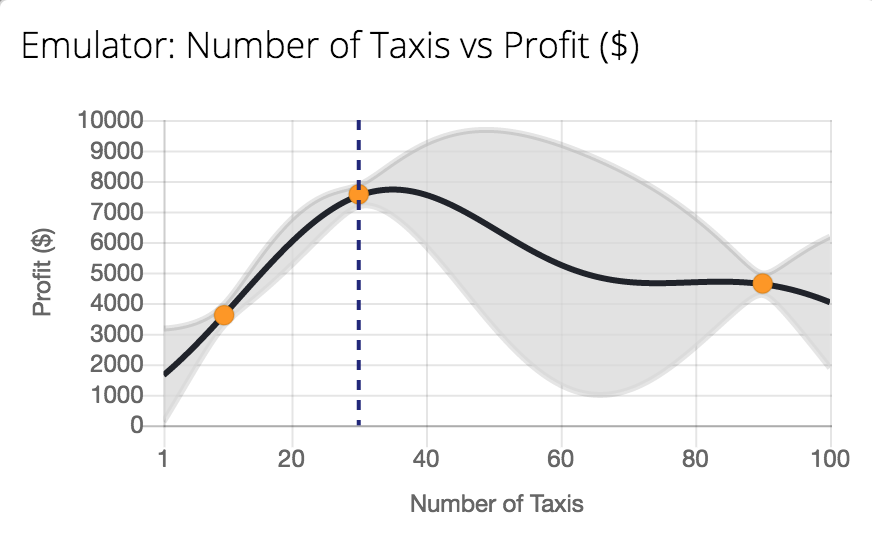
Figure: Tutorial on Bayesian optimization of the number of taxis deployed from Emukit playground. https://amzn.github.io/emukit-playground/#!/learn/bayesian_optimization

You can explore Bayesian optimization of a taxi simulation.

Emukit Tutorial

%pip install mlai

Set up the python imports that Emukit will use.

import numpy as np
import GPy

Now set up Emukit to run.

from emukit.experimental_design.experimental_design_loop import ExperimentalDesignLoop

Let’s check the help function for the experimental design loop. This is the outer loop that provides all the decision making parts of Emukit.

ExperimentalDesignLoop?

Now let’s load in the model wrapper for our probabilistic model. In this case, instead of using GPy, we’ll make use of a simple model wrapper Emukit provides for a basic form of Gaussian process.

from emukit.model_wrappers import SimpleGaussianProcessModel

Let’s have a quick look at how the included GP model works.

SimpleGaussianProcessModel?

Now let’s create the data.

x_min = -30.0
x_max = 30.0

x = np.random.uniform(x_min, x_max, (10, 1))
y = np.sin(x) + np.random.randn(10, 1) * 0.05

To learn about how to include your own model in Emukit, check this notebook which shows how to include a sklearn GP model.

emukit_model = SimpleGaussianProcessModel(x, y)

from emukit.core import ParameterSpace, ContinuousParameter
from emukit.core.loop import UserFunctionWrapper

p = ContinuousParameter('c', x_min, x_max)
space = ParameterSpace([p])

loop = ExperimentalDesignLoop(space, emukit_model)
loop.run_loop(np.sin, 30)

plot_min = -40.0
plot_max = 40.0

real_x = np.arange(plot_min, plot_max, 0.2)
real_y = np.sin(real_x)

Figure: Experimental design in Emukit using the ExperimentalDesignLoop: learning function \(\sin(x)\) with Emukit.

Computer the predictions from the Emukit model.

predicted_y = []
predicted_std = []
for x in real_x:
    y, var = emukit_model.predict(np.array([[x]]))
    std = np.sqrt(var)
    predicted_y.append(y)
    predicted_std.append(std)

predicted_y = np.array(predicted_y).flatten()
predicted_std = np.array(predicted_std).flatten()

Figure: The fit to the sine function after runnning the Emukit ExperimentalDesignLoop.

Exercise 3

Repeat the above experiment but using the Gaussian process model from sklearn. You can see step by step instructions on how to do this in this notebook.

Emukit Overview Summary

The aim is to provide a suite where different approaches to emulation are assimilated under one roof. The current version of Emukit includes multi-fidelity emulation for build surrogate models when data is obtained from multiple information sources that have different fidelity and/or cost; Bayesian optimisation for optimising physical experiments and tune parameters of machine learning algorithms or other computational simulations; experimental design and active learning: design the most informative experiments and perform active learning with machine learning models; sensitivity analysis: analyse the influence of inputs on the outputs of a given system; and Bayesian quadrature: efficiently compute the integrals of functions that are expensive to evaluate. But it’s easy to extend.

Emukit Sensitivity Analysis

This introduction is based on Introduction to Global Sensitivity Analysis with Emukit written by Mark Pullin, Javier Gonzalez, Juan Emmanuel Johnson and Andrei Paleyes. Some references include (Kennedy and O’Hagan, 2000; Saltelli et al., 2010, 2008, 2004; Sobol, 2001, 1990)

A possible definition of sensitivity analysis is the following: The study of how uncertainty in the output of a model (numerical or otherwise) can be apportioned to different sources of uncertainty in the model input (Saltelli et al., 2004). A related practice is ‘uncertainty analysis,’ which focuses rather on quantifying uncertainty in model output. Ideally, uncertainty and sensitivity analyses should be run in tandem, with uncertainty analysis preceding in current practice.

In Chapter 1 of Saltelli et al. (2008)

import numpy as np
import matplotlib.pyplot as plt

from matplotlib import colors as mcolors
from matplotlib import cm

%pip install pyDOE

import mlai
import mlai.plot as plot

Sensitivity analysis is a statistical technique widely used to test the reliability of real systems. Imagine a simulator of taxis picking up customers in a city like the one showed in the Emukit playground. The profit of the taxi company depends on factors like the number of taxis on the road and the price per trip. In this example, a global sensitivity analysis of the simulator could be useful to decompose the variance of the profit in a way that can be assigned to the input variables of the simulator.

There are different ways of doing a sensitivity analysis of the variables of a simulator. In this notebook we will start with an approach based on Monte Carlo sampling that is useful when evaluating the simulator is cheap. If evaluating the simulator is expensive, emulators can then be used to speed up computations. We will show this in the last part of the notebook. Next, we start with a few formal definitions and literature review so we can understand the basics of Sensitivity Analysis and how it can be performed with Emukit.

Local Sensitivity

Given any function, \(g(\cdot)\), we might be interested in how sensitive that function is to variations in its input space. One route to determining this is to compute the partial derivatives of that function with respect to its inputs, \[ \frac{\partial}{\partial x_i} g(\mathbf{ x}). \] The matrix of all these partial derivatives is known as the Jacobian.

These types of local sensitivity analysis can be used for determining the effect of changing an input variable around an operating point. But they don’t give us an understanding of the response of the target function to variations in the input across the domain of inputs. For this, we need to look to global sensitivity analysis.

Global Sensitivity Analysis

In global sensitivity analysis, rather than looking around a single operating point, we’re interested in the overall sensitivity of a function to its inputs, or combinations of inputs, across its entire domain. The key tool in determining this sensitivity is known as the ANOVA decomposition, or the Hoeffding-Sobol decomposition.

For global sensitivity analysis, we need to make an assumption about how inputs are going to vary to create different values of the function. The fundamental object we’re interested in is the total variance of the function, \[ \text{var}\left(g(\mathbf{ x})\right) = \left\langle g(\mathbf{ x})^2 \right\rangle _{p(\mathbf{ x})} - \left\langle g(\mathbf{ x}) \right\rangle _{p(\mathbf{ x})}^2, \] where \[ \left\langle h(\mathbf{ x}) \right\rangle _{p(\mathbf{ x})} = \int_\mathbf{ x}h(\mathbf{ x}) p(\mathbf{ x}) \text{d}\mathbf{ x} \] is the expectation of the function \(h(\mathbf{ x})\) under the density \(p(\mathbf{ x})\), which represents the probability distribution of inputs we’re interested in.

The total variance of the function gives us the overall variation of the function across the domain of inputs, as represented by the probability density, \(p(\mathbf{ x})\). Normally, we perform analysis by assuming that, \[ p(\mathbf{ x}) = \prod_{i=1}^pp(x_i) \] and that each \(p(x_i)\) is uniformly distributed across its input domain. Assuming we scale the input domain down to the interval \([0, 1]\), that gives us \[ x_i \sim \mathcal{U}\left(0,1\right). \]

Hoeffding-Sobol Decomposition

The Hoeffding-Sobol, or ANOVA, decomposition of a function allows us to write it as, \[ \begin{align*} g(\mathbf{ x}) = & g_0 + \sum_{i=1}^pg_i(x_i) + \sum_{i<j}^{p} g_{ij}(x_i,x_j) + \cdots \\ & + g_{1,2,\dots,p}(x_1,x_2,\dots,x_p), \end{align*} \] where \[ g_0 = \left\langle g(\mathbf{ x}) \right\rangle _{p(\mathbf{ x})} \] and \[ g_i(x_i) = \left\langle g(\mathbf{ x}) \right\rangle _{p(\mathbf{ x}_{\sim i})} - g_0, \] where we’re using the notation \(p(\mathbf{ x}_{\sim i})\) to represent the input distribution with the \(i\)th variable marginalised, \[ p(\mathbf{ x}_{\sim i}) = \int p(\mathbf{ x}) \text{d}x_i \] Higher order terms in the decomposition represent interactions between inputs, \[ g_{i,j}(x_i, x_j) = \left\langle g(\mathbf{ x}) \right\rangle _{p(\mathbf{ x}_{\sim i,j})} - g_i(x_i) - g_j(x_j) - g_0 \] and similar expressions can be written for higher order terms up to \(g_{1,2,\dots,p}(\mathbf{ x})\).

Note that to compute each of these individual terms, you need to first compute the low order terms, and then compute the high order terms. This can be problematic when \(p\) is large.

We’re interested in the variance of the function \(g\), so implicitly we’re assuming that the square of this function is integrable across its domain, i.e., we’re assuming that \(\left\langle g(\mathbf{ x})^2 \right\rangle _{p(\mathbf{ x})}\) exists and is finite.

The Sobol decomposition has some important properties, in particular, its components are orthogonal, so this means that when we substitute it in to the variance, we have, \[ \begin{align*} \text{var}(g) = & \left\langle g(\mathbf{ x})^2 \right\rangle _{p(\mathbf{ x})} - \left\langle g(\mathbf{ x}) \right\rangle _{p(\mathbf{ x})}^2 \\ = & \left\langle g(\mathbf{ x})^2 \right\rangle _{p(\mathbf{ x})} - g_0^2\\ = & \sum_{i=1}^p\text{var}\left(g_i(x_i)\right) + \sum_{i<j}^{p} \text{var}\left(g_{ij}(x_i,x_j)\right) + \cdots \\ & + \text{var}\left(g_{1,2,\dots,p}(x_1,x_2,\dots,x_p)\right). \end{align*} \] So, this decomposition gives us a decomposition of the function in terms of variances. It’s for this reason that it’s sometimes known as an ANOVA decomposition. ANOVA stands a for analysis of variance. The ANOVA decomposition decomposes the function into additive variance parts that are each stemming from interactions between different inputs.

As is common in various analyses of variance, we can rescale the components with the total variance of the function. These rescaled components are known as Sobol indicies. \[ S_\ell = \frac{\text{var}\left(g(\mathbf{ x}_\ell)\right)}{\text{var}\left(g(\mathbf{ x})\right)}, \] where the \(\ell\) represents the relevent set of indices for the different combinations of inputs.

In practice, for an elegant approach that exploits a particular covariance function structure to perform global sensitivity analysis see Durrande et al. (2013).

Example: the Ishigami function

We illustrate the exact calculation of the Sobol indices with the three-dimensional Ishigami function of (Ishigami and Homma, 1989).

Ishigami Function

The Ishigami function (Ishigami and Homma, 1989) is a well-known test function for uncertainty and sensitivity analysis methods because of its strong nonlinearity and peculiar dependence on \(x_3\). More details of this function can be found in (Sobol and Levitan, 1999).

Mathematically, the form of the Ishigami function is \[ g(\textbf{x}) = \sin(x_1) + a \sin^2(x_2) + b x_3^4 \sin(x_1). \] We will set the parameters to be \(a = 5\) and \(b=0.1\) . The input variables are sampled randomly \(x_i \sim \mathcal{U}\left(-\pi,\pi\right)\).

Next, we create the function object and visualize its shape marginally for each one of its three inputs.

Load the Ishigami function

from emukit.test_functions.sensitivity import Ishigami

ishigami = Ishigami(a=5, b=0.1)
target_function = ishigami.fidelity1

That gives us the target function, next we define the input space for the simulator.

import numpy as np
from emukit.core import ContinuousParameter, ParameterSpace

variable_domain = (-np.pi,np.pi)
           
space = ParameterSpace(
          [ContinuousParameter('x1', *variable_domain), 
           ContinuousParameter('x2', *variable_domain),
           ContinuousParameter('x3', *variable_domain)])

Before moving to any further analysis, we first plot the non-zero components \(g(\mathbf{ x})\). These components are \[ \begin{align*} g_1(x_1) & = \sin(x_1) \\ g_2(x_2) & = a \sin^2 (x_2) \\ g_{13}(x_1,x_3) & = b x_3^4 \sin(x_1) \end{align*} \]

x_grid = np.linspace(*variable_domain,100)
target_simulator = ishigami.fidelity1
f1 = ishigami.f1(x_grid)
f2 = ishigami.f2(x_grid)
F13 = ishigami.f13(np.array([x_grid,x_grid]).T)[:,np.newaxis]

Figure: The non-zero components of the Ishigami function.

Total Variance

The total variance \(\text{var}(y)\) in this example is

print(ishigami.variance_total)

which is the sum of the variance of \(\text{var}\left(g_1(x_1)\right)\), \(\text{var}\left(g_2(x_2)\right)\) and \(\text{var}\left(g_{1,3}(x_{1,3})\right)\)

print(ishigami.variance_x1, ishigami.variance_x2, ishigami.variance_x13)
print(ishigami.variance_x1 + ishigami.variance_x2 + ishigami.variance_x13)

First Order Sobol Indices using Monte Carlo

The first order Sobol indices are a measure of “first order sensitivity” of each input variable. They account for the proportion of variance of \(y\) explained by changing each variable alone while marginalizing over the rest. Recall that the Sobol index of the \(i\)th variable is computed as \[ S_i = \frac{\text{var}\left(g_i(x_i)\right)}{\text{var}\left(g(\mathbf{ x})\right)}. \] This value is standardized using the total variance, so it is possible to account for a fractional contribution of each variable to the total variance of the output.

The Sobol indices for higher order interactions \(S_{i,j}\) are computed similarly. Due to the normalization by the total variance, the the sum of all Sobol indices equals to one.

In most cases we are interested in the first order indices. The Ishigami function has the benefit that these can be computed analytically. In EmuKit you can extract these values with the code.

ishigami.main_effects

But in general, these indices need to be sampled using Monte Carlo or one of the quasi-Monte Carlo methods we’ve seen in the model-free experimental design. Details are given in (Sobol, 2001).

With Emukit, the first-order Sobol indices can be easily computed. We first need to define the space where the target simulator is analyzed.

from emukit.sensitivity.monte_carlo import ModelFreeMonteCarloSensitivity

np.random.seed(10)  # for reproducibility

num_monte_carlo_points = 10000  # Number of MC samples
senstivity_ishigami = ModelFreeMonteCarloSensitivity(target_simulator, space)
main_effects, total_effects, _ = senstivity_ishigami.compute_effects(num_monte_carlo_points = num_monte_carlo_points)
print(main_effects)

We compare the true effects with the Monte Carlo effects in a bar-plot. The total effects are discussed later.

Figure: The non-zero components of the Ishigami function.

Total Effects Using Monte Carlo

Computing high order sensitivity indices can be computationally very demanding in high dimensional scenarios and measuring the total influence of each variable on the variance of the output is infeasible. To solve this issue the total indices are used which account for the contribution to the output variance of \(x_i\) including all variance caused by the variable alone and all its interactions of any order.

The total effect for \(x_i\) is given by: \[ S_{Ti} = \frac{\left\langle \text{var}_{x_i} (y\mid \mathbf{ x}_{\sim i}) \right\rangle _{p(\mathbf{ x}_{\sim i})}}{\text{var}\left(g(\mathbf{ x})\right)} = 1 - \frac{\text{var}_{\mathbf{ x}_{\sim i}} \left\langle y\mid \mathbf{ x}_{\sim i} \right\rangle _{p(\mathbf{ x}_{\sim i})}}{\text{var}\left(g(\mathbf{ x})\right)} \]

Note that the sum of \(S_{Ti}\) is not necessarily one in this case unless the model is additive. In the Ishigami example the value of the total effects is

ishigami.total_effects

As in the previous example, the total effects can be computed with Monte Carlo. In the next plot we show the comparison with the true total effects.

Figure: The total effects from the Ishigami function as computed via Monte Carlo estimate alongside the true total effects for the Ishigami function.

Computing the Sensitivity Indices Using the Output of a Model

In the example used above the Ishigami function is very cheap to evaluate. However, in most real scenarios the functions of interest are expensive, and we need to limit ourselves to a few number of evaluations. Using Monte Carlo methods is infeasible in these scenarios as a large number of samples are typically required to provide good estimates of the Sobol indices.

An alternative in these cases is to use Gaussaian process emulator of the function of interest trained on a few inputs and outputs (Marrel et al., 2009). If the model is properly trained, its mean prediction which is cheap to evaluate, can be used to compute the Monte Carlo estimates of the Sobol indices, the variance from the GP emulator can also be used to assess our uncertainty about the Sobol indices. Let’s see how we can do this in Emukit.

We start by generating 100 samples in the input domain. Note that this a just 1% of the number of samples that we used to compute the Sobol coefficients using Monte Carlo.

from emukit.core.initial_designs import RandomDesign

design = RandomDesign(space)
x = design.get_samples(500)
y = ishigami.fidelity1(x)[:,np.newaxis]

Now, we fit a standard Gaussian process to the samples, and we wrap it as an Emukit model.

from GPy.models import GPRegression
from emukit.model_wrappers import GPyModelWrapper
from emukit.sensitivity.monte_carlo import MonteCarloSensitivity

model_gpy = GPRegression(x,y)
model_emukit = GPyModelWrapper(model_gpy)
model_emukit.optimize()

The final step is to compute the coefficients using the class ModelBasedMonteCarloSensitivity which directly calls the model and uses its predictive mean to compute the Monte Carlo estimates of the Sobol indices. We plot the true estimates, those computed using 10000 direct evaluations of the object using Monte Carlo and those computed using a Gaussian process model trained on 100 evaluations.

num_mc = 10000
senstivity_ishigami_gpbased = MonteCarloSensitivity(model = model_emukit, input_domain = space)
main_effects_gp, total_effects_gp, _ = senstivity_ishigami_gpbased.compute_effects(num_monte_carlo_points = num_mc)

Figure: First order Sobol indices as estimated by Monte Carlo and GP-emulator based Monte Carlo.

Figure: Total effects as estimated by Monte Carlo and GP based Monte Carlo.

We observe some discrepancies with respect to the real value of the Sobol index when using the Gaussian process, but we get a fairly good approximation with a very reduced number of evaluations of the original target function.

Conclusions

The Sobol indices are a tool for explaining the variance of the output of a function as components of the input variables. Monte Carlo is an approach for computing these indices if the function is cheap to evaluate. Other approaches are needed when \(g(\cdot)\) is expensive to compute.

Catapult Simulation

As a worked example we’re going to introduce a catapult simulation written by Nicolas Durrande, https://durrande.shinyapps.io/catapult/.

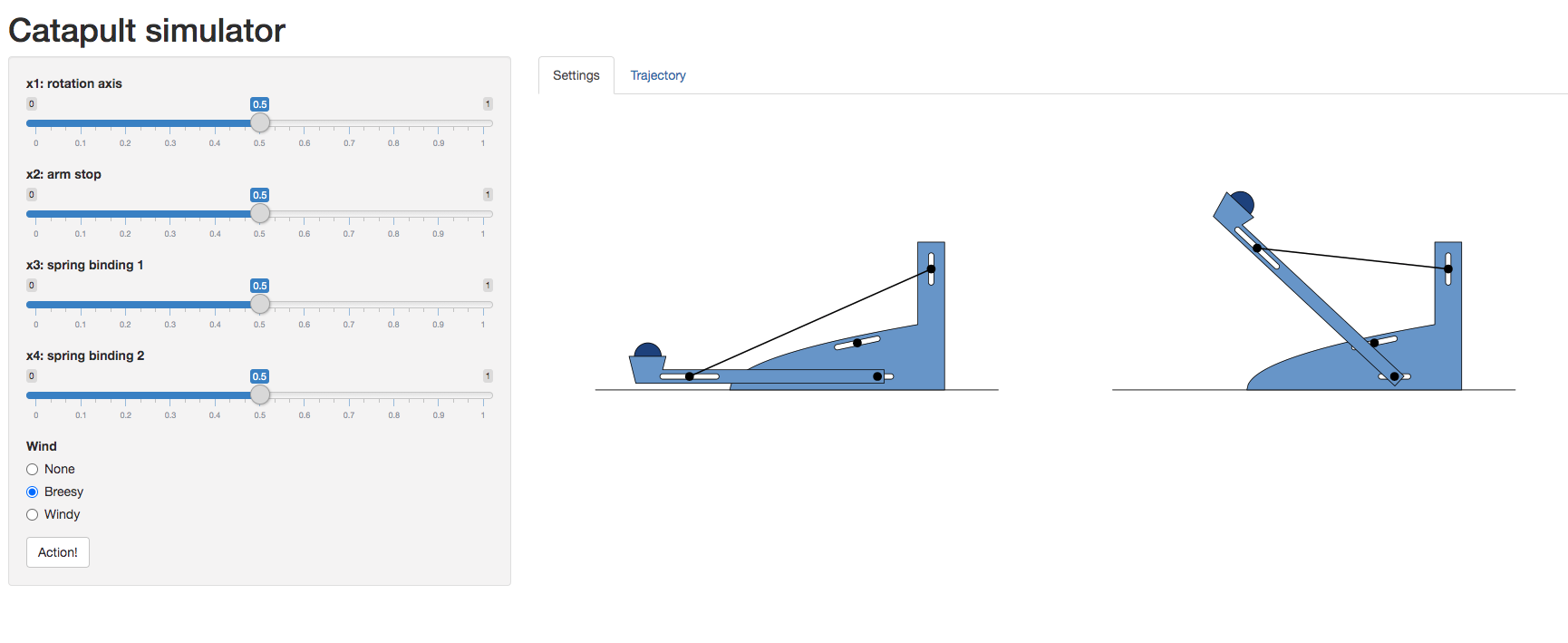
Figure: A catapult simulation for experimenting with surrogate models, kindly provided by Nicolas Durrande

The simulator allows you to set various parameters of the catapult including the axis of rotation, roation_axis, the position of the arm stop, arm_stop, and the location of the two bindings of the catapult’s spring, spring_binding_1 and spring_binding_2.

These parameters are then collated in a vector, \[ \mathbf{ x}_i = \begin{bmatrix} \texttt{rotation_axis} \\ \texttt{arm_stop} \\ \texttt{spring_binding_1} \\ \texttt{spring_binding_2} \end{bmatrix} \]

Having set those parameters, you can run an experiment, by firing the catapult. This will show you how far it goes.

Because you will need to operate the catapult yourself, we’ll create a function to query you about the result of an individual firing.

We can also set the parameter space for the model. Each of these variables is scaled to operate \(\in [0, 1]\).

from emukit.core import ContinuousParameter, ParameterSpace

variable_domain = [0,1]
           
space = ParameterSpace(
          [ContinuousParameter('rotation_axis', *variable_domain), 
           ContinuousParameter('arm_stop', *variable_domain),
           ContinuousParameter('spring_binding_1', *variable_domain),
           ContinuousParameter('spring_binding_2', *variable_domain)])

Before we perform sensitivity analysis, we need to build an emulator of the catapulter, which we do using our experimental design process.

Experimental Design for the Catapult

Now we will build an emulator for the catapult using the experimental design loop.

We’ll start with a small model-free design, we’ll use a random design for initializing our model.

from emukit.core.initial_designs import RandomDesign

design = RandomDesign(space)
x = design.get_samples(5)
y = catapult_distance(x)

from GPy.models import GPRegression
from emukit.model_wrappers import GPyModelWrapper
from emukit.sensitivity.monte_carlo import MonteCarloSensitivity

Set up the GPy model. The variance of the RBF kernel is set to \(150^2\) because that’s roughly the square of the range of the catapult. We set the noise variance to a small value.

model_gpy = GPRegression(x,y)
model_gpy.kern.variance = 150**2
model_gpy.likelihood.variance.fix(1e-5)
display(model_gpy)

Wrap the model for EmuKit.

model_emukit = GPyModelWrapper(model_gpy)
model_emukit.optimize()

display(model_gpy)

Now we set up the model loop. We’ll use integrated variance reduction as the acquisition function for our model-based design loop.

Warning: This loop runs much slower on Google colab than on a local machine.

from emukit.experimental_design.experimental_design_loop import ExperimentalDesignLoop

from emukit.experimental_design.acquisitions import IntegratedVarianceReduction, ModelVariance

integrated_variance = IntegratedVarianceReduction(space=space,
                                                  model=model_emukit)
ed = ExperimentalDesignLoop(space=space, 
                            model=model_emukit, 
                            acquisition = integrated_variance)
ed.run_loop(catapult_distance, 10)

Sensitivity Analysis of a Catapult Simulation

The final step is to compute the coefficients using the class ModelBasedMonteCarloSensitivity which directly calls the model and uses its predictive mean to compute the Monte Carlo estimates of the Sobol indices. We plot the estimates of the Sobol indices computed using a Gaussian process model trained on the observations we’ve acquired.

num_mc = 10000
senstivity = MonteCarloSensitivity(model = model_emukit, input_domain = space)
main_effects_gp, total_effects_gp, _ = senstivity.compute_effects(num_monte_carlo_points = num_mc)

Figure: First Order sobol indices as estimated by GP-emulator based Monte Carlo on the catapult.

Figure: Total effects as estimated by GP based Monte Carlo on the catapult.

Thanks!

For more information on these subjects and more you might want to check the following resources.

• twitter: @lawrennd
• podcast: The Talking Machines
• newspaper: Guardian Profile Page
• blog: http://inverseprobability.com

References