Il nucleo umano
Links
Abstract
A vital perspective is missing from the discussions we’re having about Artificial Intelligence: what does it mean for our identity?
Our fascination with AI stems from the perceived uniqueness of human intelligence. We believe it’s what differentiates us. Fears of AI not only concern how it invades our digital lives, but also the implied threat of an intelligence that displaces us from our position at the centre of the world.
Atomism, proposed by Democritus, suggested it was impossible to continue dividing matter down into ever smaller components: eventually we reach a point where a cut cannot be made (the Greek for uncuttable is ‘atom’). In the same way, by slicing away at the facets of human intelligence that can be replaced by machines, AI uncovers what is left: an indivisible core that is the essence of humanity.
I’ll contrast our own (evolved, locked-in, embodied) intelligence with the capabilities of machine intelligence and speculate on what it means for our futures — including for communities that are too often left out of cultural and educational exchange about these technologies.
This talk is based on Neil’s book The Atomic Human, available in Italian as Il nucleo umano.
Henry Ford’s Faster Horse

Figure: A 1925 Ford Model T built at Henry Ford’s Highland Park Plant in Dearborn, Michigan. This example now resides in Australia, owned by the founder of FordModelT.net. From https://commons.wikimedia.org/wiki/File:1925_Ford_Model_T_touring.jpg

It’s said that Henry Ford’s customers wanted a “a faster horse.” If Henry Ford was selling us artificial intelligence today, what would the customer call for, “a smarter human?” That’s certainly the picture of machine intelligence we find in science fiction narratives, but the reality of what we’ve developed is much more mundane.
Car engines produce prodigious power from petrol. Machine intelligences deliver decisions derived from data. In both cases the scale of consumption enables a speed of operation that is far beyond the capabilities of their natural counterparts. Unfettered energy consumption has consequences in the form of climate change. Does unbridled data consumption also have consequences for us?
If we devolve decision making to machines, we depend on those machines to accommodate our needs. If we don’t understand how those machines operate, we lose control over our destiny. Our mistake has been to see machine intelligence as a reflection of our intelligence. We cannot understand the smarter human without understanding the human. To understand the machine, we need to better understand ourselves.
Artificial General Vehicle
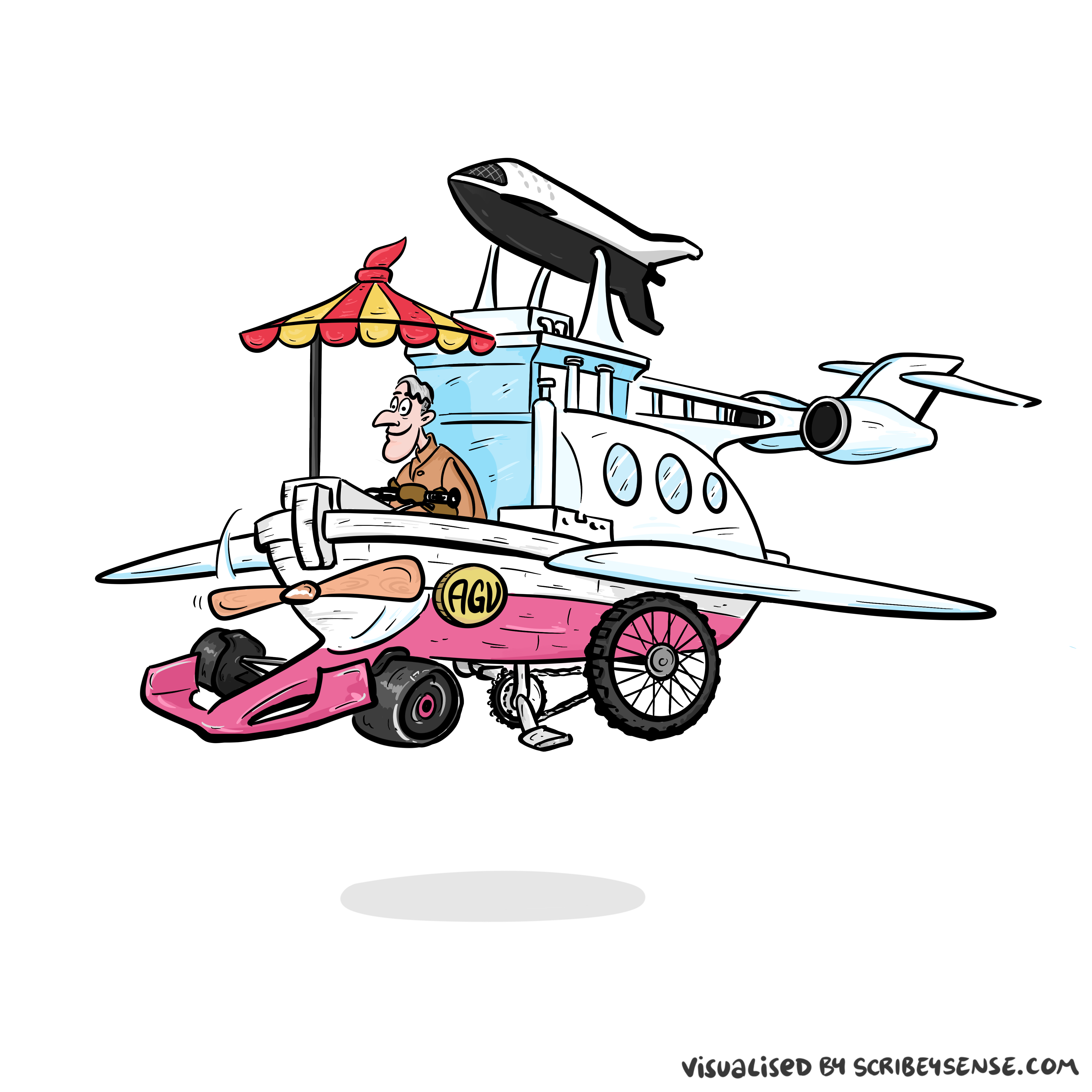
Figure: The notion of artificial general intelligence is as absurd as the notion of an artificial general vehicle - no single vehicle is optimal for every journey. (Illustration by Dan Andrews inspired by a conversation about “The Atomic Human” Lawrence (2024))
This illustration was created by Dan Andrews inspired by a conversation about “The Atomic Human” book. The drawing emerged from discussions with Dan about the flawed concept of artificial general intelligence and how it parallels the absurd idea of a single vehicle optimal for all journeys. The vehicle itself is inspired by shared memories of Professor Pat Pending in Hanna Barbera’s Wacky Races.
I often turn up to talks with my Brompton bicycle. Embarrassingly I even took it to Google which is only a 30 second walk from King’s Cross station. That made me realise it’s become a sort of security blanket. I like having it because it’s such a flexible means of transport.
But is the Brompton an “artificial general vehicle?” A vehicle that can do everything? Unfortunately not, for example it’s not very good for flying to the USA. There is no artificial general vehicle that is optimal for every journey. Similarly there is no such thing as artificial general intelligence. The idea is artificial general nonsense.
That doesn’t mean there aren’t different principles to intelligence we can look at. Just like vehicles have principles that apply to them. When designing vehicles we need to think about air resistance, friction, power. We have developed solutions such as wheels, different types of engines and wings that are deployed across different vehicles to achieve different results.
Intelligence is similar. The notion of artificial general intelligence is fundamentally eugenic. It builds on Spearman’s term “general intelligence” which is part of a body of literature that was looking to assess intelligence in the way we assess height. The objective then being to breed greater intelligences (Lyons, 2022).
The Atomic Human
Figure: The Atomic Eye, by slicing away aspects of the human that we used to believe to be unique to us, but are now the preserve of the machine, we learn something about what it means to be human.
The development of what some are calling intelligence in machines, raises questions around what machine intelligence means for our intelligence. The idea of the atomic human is derived from Democritus’s atomism.
In the fifth century bce the Greek philosopher Democritus posed a question about our physical universe. He imagined cutting physical matter into pieces in a repeated process: cutting a piece, then taking one of the cut pieces and cutting it again so that each time it becomes smaller and smaller. Democritus believed this process had to stop somewhere, that we would be left with an indivisible piece. The Greek word for indivisible is atom, and so this theory was called atomism.
The Atomic Human considers the same question, but in a different domain, asking: As the machine slices away portions of human capabilities, are we left with a kernel of humanity, an indivisible piece that can no longer be divided into parts? Or does the human disappear altogether? If we are left with something, then that uncuttable piece, a form of atomic human, would tell us something about our human spirit.
See Lawrence (2024) atomic human, the p. 13.
Embodiment Factors: Walking vs Light Speed
Imagine human communication as moving at walking pace. The average person speaks about 160 words per minute, which is roughly 2000 bits per minute. If we compare this to walking speed, roughly 1 m/s we can think of this as the speed at which our thoughts can be shared with others.
Compare this to machines. When computers communicate, their bandwidth is 600 billion bits per minute. Three hundred million times faster than humans or the equiavalent of \(3 \times 10 ^{8}\). In twenty minutes we could be a kilometer down the road, where as the computer can go to the Sun and back again..
This difference is not just only about speed of communication, but about embodiment. Our intelligence is locked in by our biology: our brains may process information rapidly, but our ability to share those thoughts is limited to the slow pace of speech or writing. Machines, in comparison, seem able to communicate their computations almost instantaneously, anywhere.
So, the embodiment factor is the ratio between the time it takes to think a thought and the time it takes to communicate it. For us, it’s like walking; for machines, it’s like moving at light speed. This difference means that most direct comparisons between human and machine need to be carefully made. Because for humans not the size of our communication bandwidth that counts, but it’s how we overcome that limitation..
Figure: Conversation relies on internal models of other individuals.
Figure: Misunderstanding of context and who we are talking to leads to arguments.
Embodiment factors imply that, in our communication between humans, what is not said is, perhaps, more important than what is said. To communicate with each other we need to have a model of who each of us are.
To aid this, in society, we are required to perform roles. Whether as a parent, a teacher, an employee or a boss. Each of these roles requires that we conform to certain standards of behaviour to facilitate communication between ourselves.
Control of self is vitally important to these communications.
The consequences between this mismatch of power and delivery are to be seen all around us. Because, just as driving an F1 car with bicycle wheels would be a fine art, so is the process of communication between humans.
If I have a thought and I wish to communicate it, I first need to have a model of what you think. I should think before I speak. When I speak, you may react. You have a model of who I am and what I was trying to say, and why I chose to say what I said. Now we begin this dance, where we are each trying to better understand each other and what we are saying. When it works, it is beautiful, but when mis-deployed, just like a badly driven F1 car, there is a horrible crash, an argument.
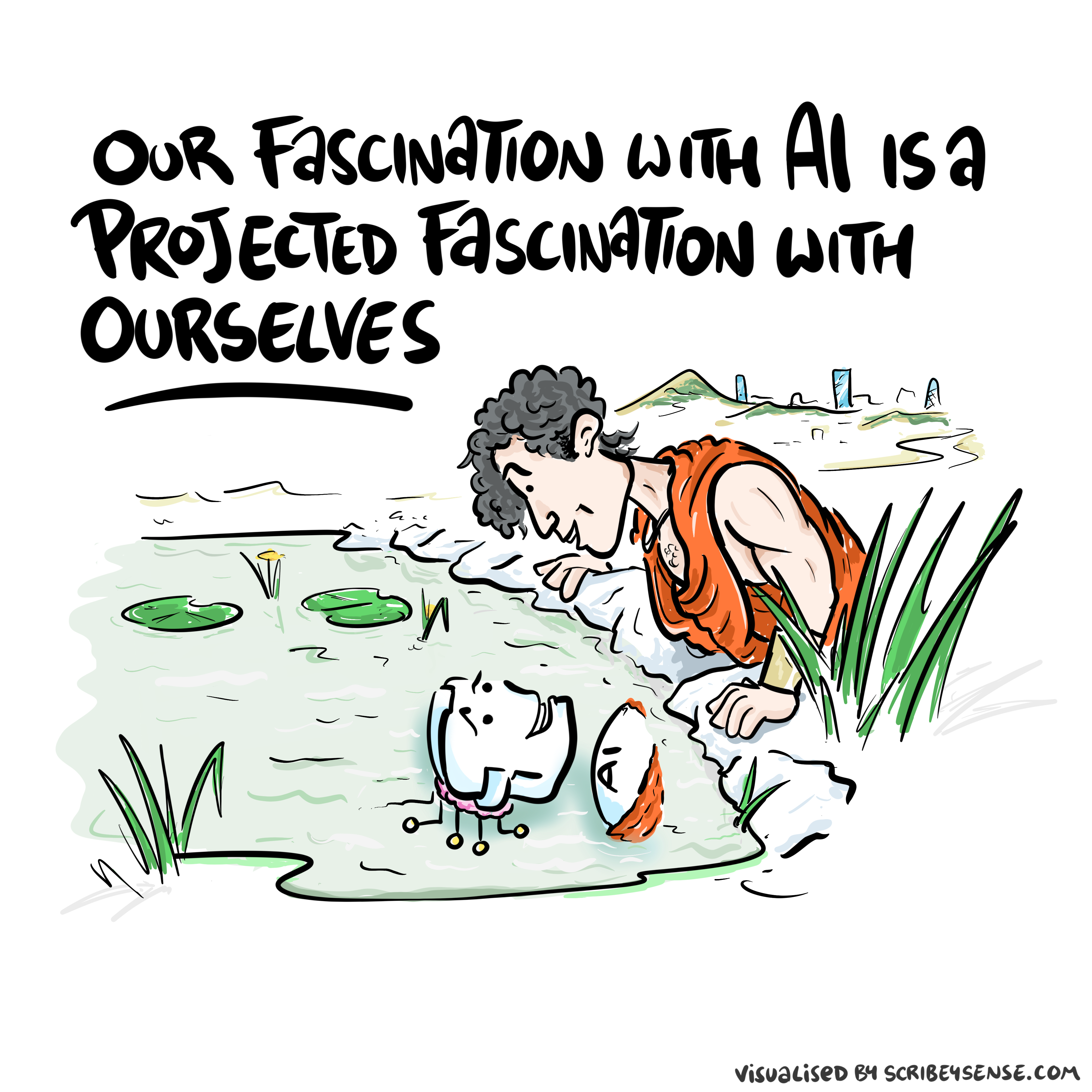
Figure: This is the drawing Dan was inspired to create for Chapter 1. It captures the fundamentally narcissistic nature of our (societal) obsession with our intelligence.
See blog post on Dan Andrews image of our reflective obsession with AI.. See also (Vallor, 2024).
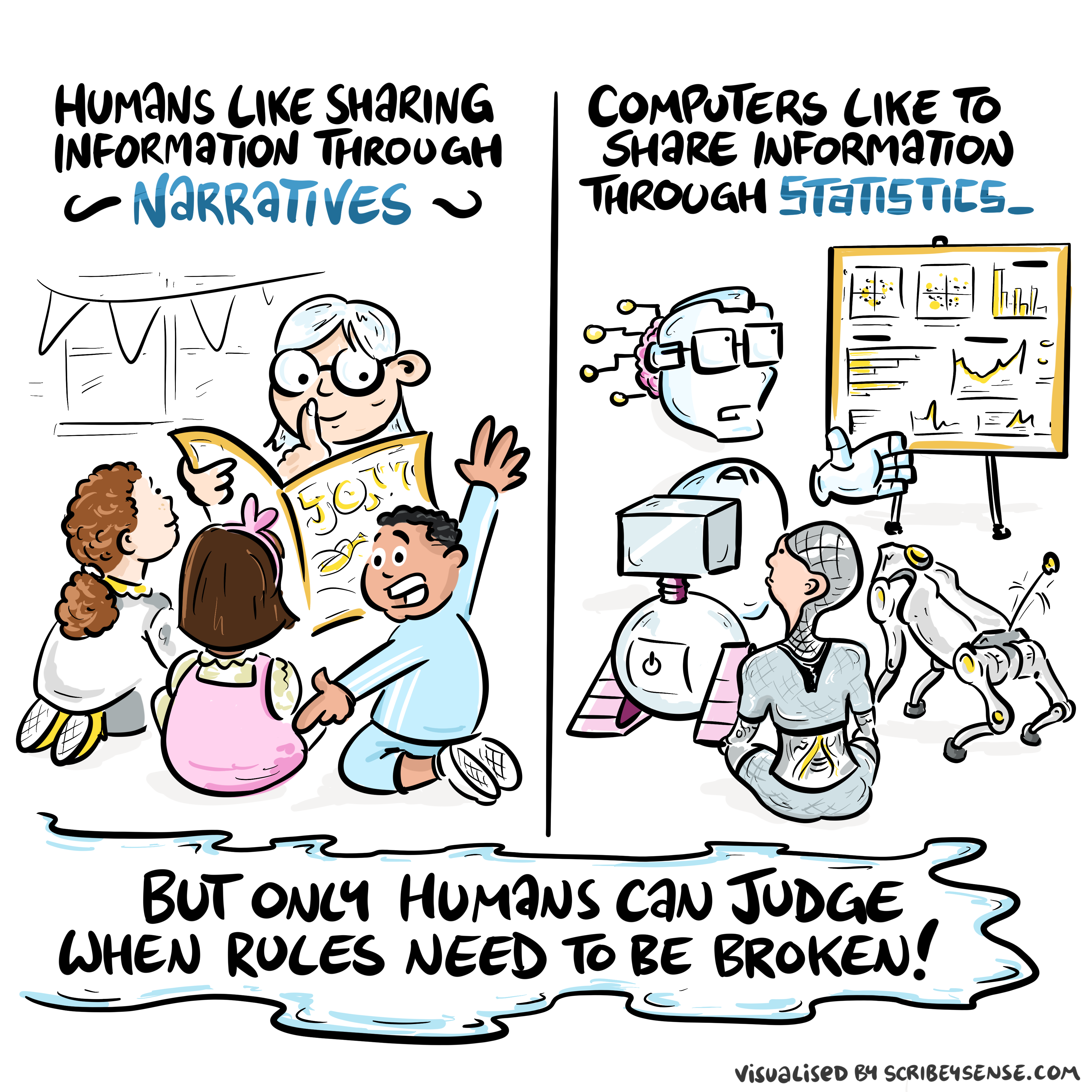
Figure: This is the drawing Dan was inspired to create for Chapter 2. It captures part of the narrative where human actors choose to follow the spirit of their instructions, and are empowered to do so because they have wider context. They can operate autonomously. Whereas machines have typically operated on data and statistics and can’t bring in context so normally operate as automatons.
See blog post on Dan Andrews image of narratives vs statistics..
New Flow of Information
Classically the field of statistics focused on mediating the relationship between the machine and the human. Our limited bandwidth of communication means we tend to over-interpret the limited information that we are given, in the extreme we assign motives and desires to inanimate objects (a process known as anthropomorphizing). Much of mathematical statistics was developed to help temper this tendency and understand when we are valid in drawing conclusions from data.
Figure: The trinity of human, data, and computer, and highlights the modern phenomenon. The communication channel between computer and data now has an extremely high bandwidth. The channel between human and computer and the channel between data and human is narrow. New direction of information flow, information is reaching us mediated by the computer. The focus on classical statistics reflected the importance of the direct communication between human and data. The modern challenges of data science emerge when that relationship is being mediated by the machine.
Data science brings new challenges. In particular, there is a very large bandwidth connection between the machine and data. This means that our relationship with data is now commonly being mediated by the machine. Whether this is in the acquisition of new data, which now happens by happenstance rather than with purpose, or the interpretation of that data where we are increasingly relying on machines to summarize what the data contains. This is leading to the emerging field of data science, which must not only deal with the same challenges that mathematical statistics faced in tempering our tendency to over interpret data but must also deal with the possibility that the machine has either inadvertently or maliciously misrepresented the underlying data.
See Lawrence (2024) topography, information p. 34-9, 43-8, 57, 62, 104, 115-16, 127, 140, 192, 196, 199, 291, 334, 354-5. See Lawrence (2024) anthropomorphization (‘anthrox’) p. 30-31, 90-91, 93-4, 100, 132, 148, 153, 163, 216-17, 239, 276, 326, 342.
Their Data Comes from Us
Stochastic Parrots
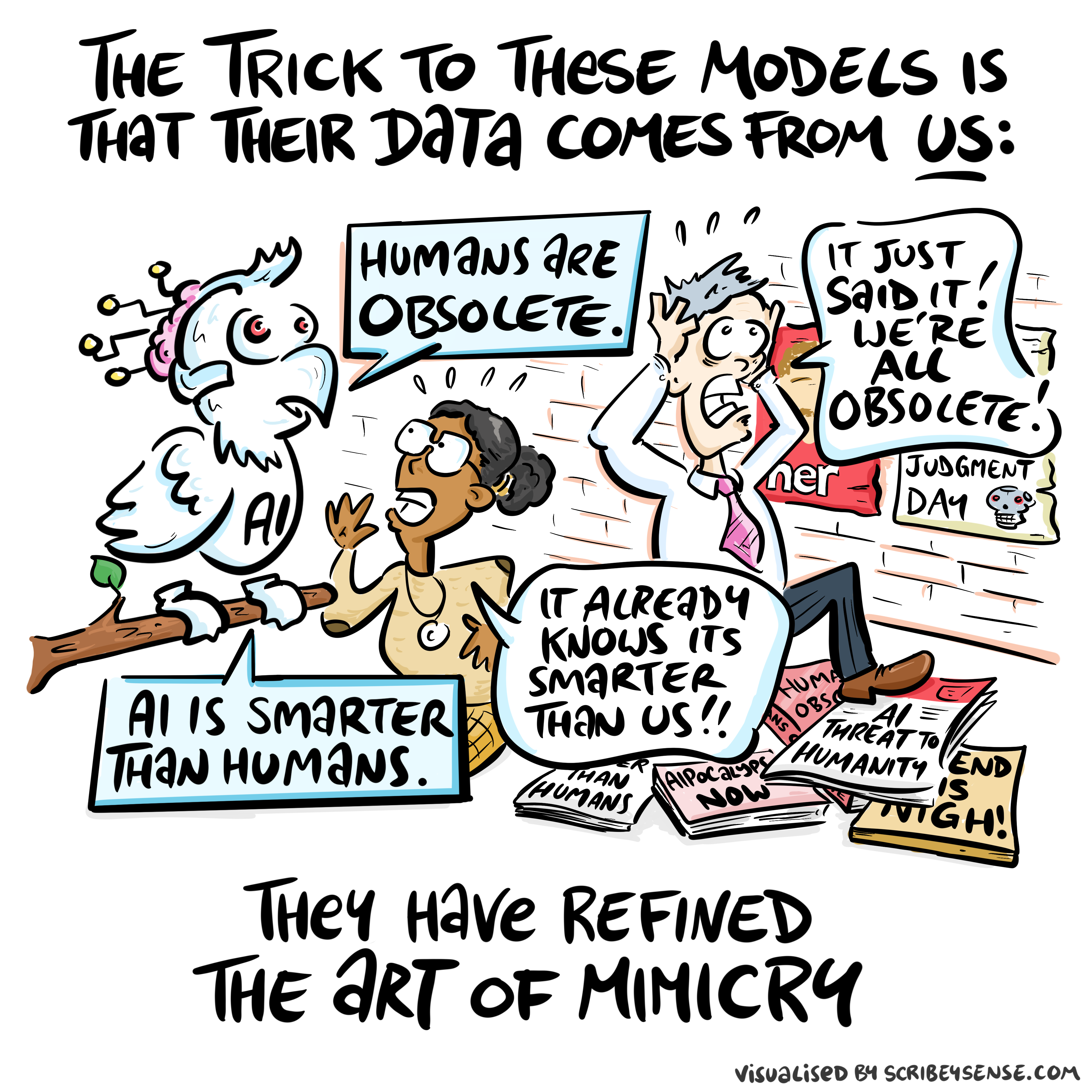
Figure: The nature of digital communication has changed dramatically, with machines processing vast amounts of human-generated data and feeding it back to us in ways that can distort our information landscape. (Illustration by Dan Andrews inspired by Chapter 5 “Enlightenment” of “The Atomic Human” Lawrence (2024))
This illustration was created by Dan Andrews after reading Chapter 5 “Enlightenment” of “The Atomic Human” book. The chapter examines how machine learning models like GPTs ingest vast amounts of human-created data and then reflect modified versions back to us. The drawing celebrates the stochastic parrots paper by Bender et al. (2021) while also capturing how this feedback loop of information can distort our digital discourse.
See blog post on Two Types of Stochastic Parrots.
The stochastic parrots paper (Bender et al., 2021) was the moment that the research community, through a group of brave researchers, some of whom paid with their jobs, raised the first warnings about these technologies. Despite their bravery, at least in the UK, their voices and those of many other female researchers were erased from the public debate around AI.
Their voices were replaced by a different type of stochastic parrot, a group of “fleshy GPTs” that speak confidently and eloquently but have little experience of real life and make arguments that, for those with deeper knowledge are flawed in naive and obvious ways.
The story is a depressing reflection of a similar pattern that undermined the UK computer industry Hicks (2018).
We all have a tendency to fall into the trap of becoming fleshy GPTs, and the best way to prevent that happening is to gather diverse voices around ourselves and take their perspectives seriously even when we might instinctively disagree.
Sunday Times article “Our lives may be enhanced by AI, but Big Tech just sees dollar signs”
Times article “Don’t expect AI to just fix everything, professor warns”
A Six Word Novel

Figure: Consider the six-word novel, apocryphally credited to Ernest Hemingway, “For sale: baby shoes, never worn.” To understand what that means to a human, you need a great deal of additional context. Context that is not directly accessible to a machine that has not got both the evolved and contextual understanding of our own condition to realize both the implication of the advert and what that implication means emotionally to the previous owner.
See Lawrence (2024) baby shoes p. 368.
But this is a very different kind of intelligence than ours. A computer cannot understand the depth of the Ernest Hemingway’s apocryphal six-word novel: “For Sale, Baby Shoes, Never worn,” because it isn’t equipped with that ability to model the complexity of humanity that underlies that statement.
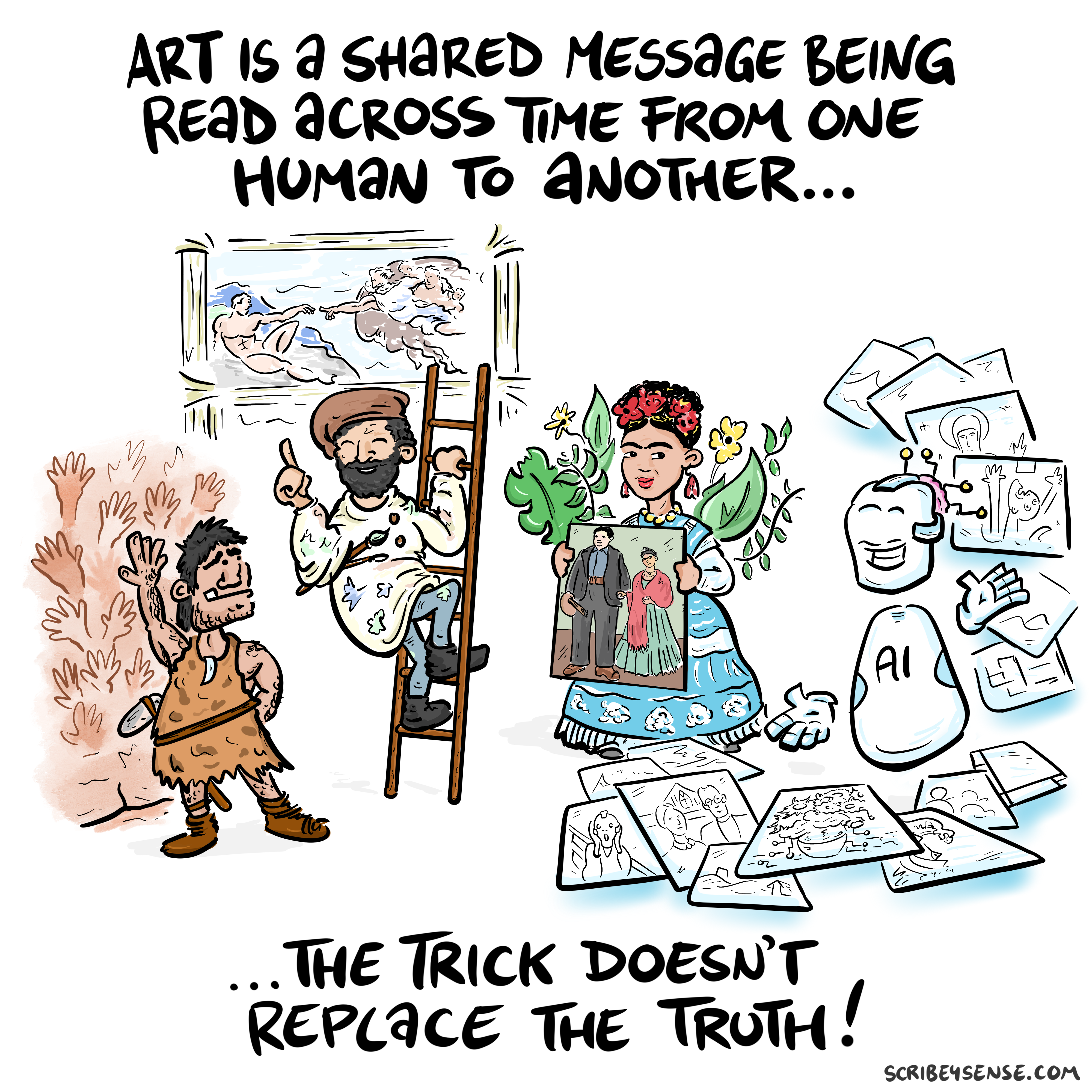
Figure: This is the drawing Dan was inspired to create for Chapter 4. It highlights how even if these machines can generate creative works the lack of origin in humans menas it is not the same as works of art that come to us through history.
See blog post on Art is Human..
For the Working Group for the Royal Society report on Machine Learning, back in 2016, the group worked with Ipsos MORI to engage in public dialogue around the technology. Ever since I’ve been struck about how much more sensible the conversations that emerge from public dialogue are than the breathless drivel that seems to emerge from supposedly more informed individuals.
There were a number of messages that emerged from those dialogues, and many of those messages were reinforced in two further public dialogues we organised in September.
However, there was one area we asked about in 2017, but we didn’t ask about in 2024. That was an area where the public unequivocal that they didn’t want the research community to pursue progress. Quoting from the report (my emphasis).
Art: Participants failed to see the purpose of machine learning-written poetry. For all the other case studies, participants recognised that a machine might be able to do a better job than a human. However, they did not think this would be the case when creating art, as doing so was considered to be a fundamentally human activity that machines could only mimic at best.
Public Views of Machine Learning, April, 2017
How right they were.
For a community audience in Acilia: keep the Atomic Human arc clear and concrete. Emphasise that debates about AI identity and agency belong outside elite centres as well — and that judgment, trust, and accountability are local as well as technical questions. Trim the Naples culture/art sequence unless the slot is long.
Thanks!
For more information on these subjects and more you might want to check the following resources.
- company: Trent AI
- book: The Atomic Human
- twitter: @lawrennd
- podcast: The Talking Machines
- newspaper: Guardian Profile Page
- blog: http://inverseprobability.com