Abstract

What is fundamental to our intelligence? In this talk building on the ideas in The Atomic Human I argue that the external world is key to our intelligence, and how that world is filtered before we perceive it. This leads to the Eisenhower illusion, where we feel ourselves in charge but we are in fact reliant on fast reacting systems.

The Blue Marble

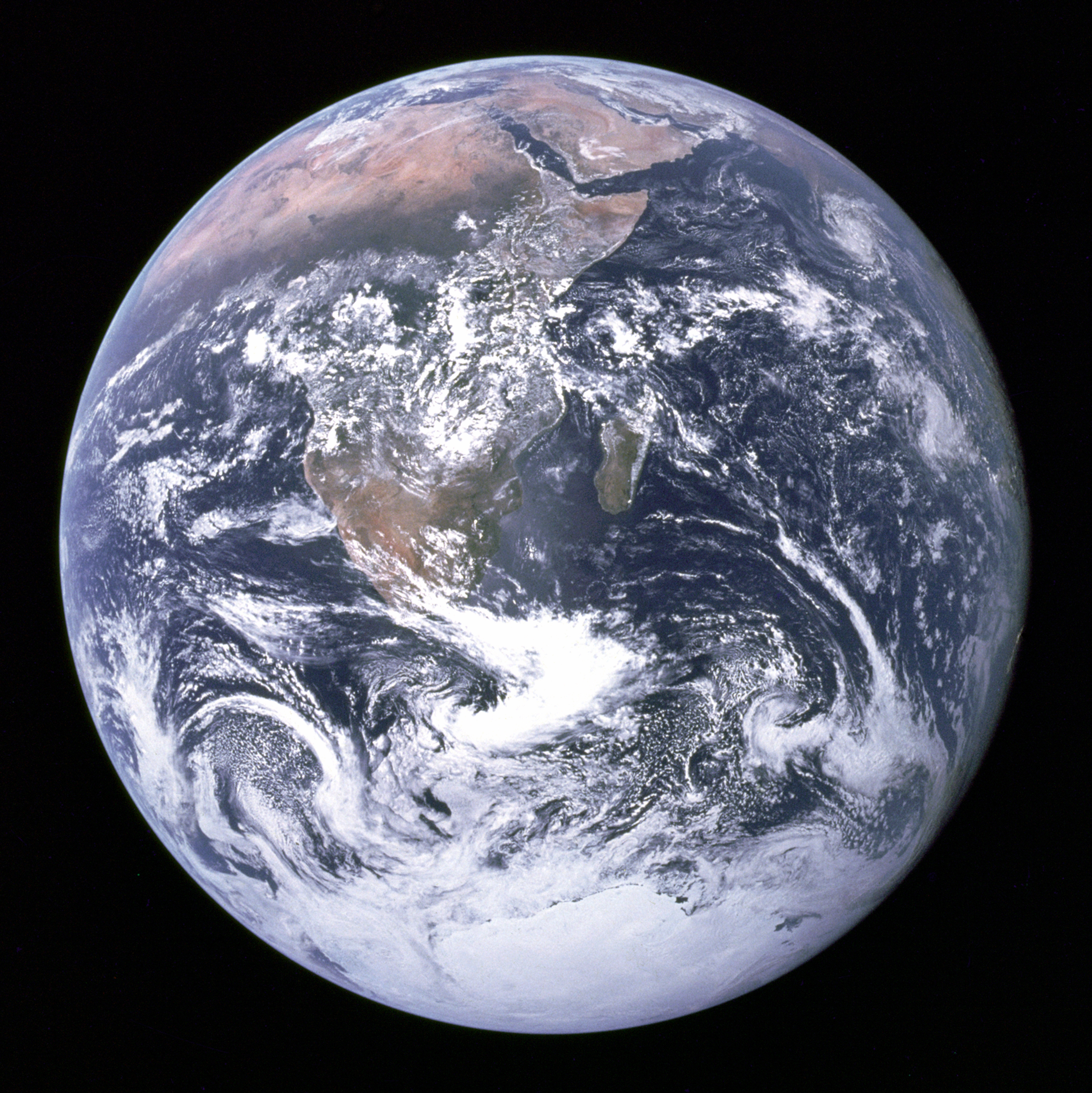
Figure: The Blue Marble, a photo of Earth taken from Apollo 17.

The Blue Marble image of the earth taken from Apollo 17 which became a symbol of the environmental movement. The photo was taken in December 1972. It gave us context. An ability to move beyond our observer bias and see us as we are. Isolated, fragile, and alone. Clinging to a rock orbiting the sun.

Eagle from Columbia

This picture, taken by Michael Collins aboard the Columbia command module, of Eagle’s return from the Moon, with the Earth in the background highlights the rendezvous radar used to to allow the crafts to dock.

See Lawrence (2024) Blue Marble (photograph) p. 367.

That radar was one sensing part of Eagle’s many automated systems (Mindell, 2008). These systems could have allowed Eagle to land without human intervention, but Armstrong chose to manually place Eagle in the Sea of Tranquility to avoid a boulder field.

The Apollo Guidance Computer mediated Armstrong’s commands, provided through a joystick, allowing him to control the craft when he input but not providing any direct connection between him and the thrusters.

Figure: Eagle photographed from Columbia on its return from the Lunar surface.

See Lawrence (2024) Apollo 11 p. 202-210.

Amelia Earhart

On 20th May 1932 Amelia Earhart took off in her Lockheed Vega from Harbour Grace in Canada. She called her plane the ‘Little Red Bus’. She travelled 2000 miles across open ocean, travelling through a storm, facing flames from her exhaust manifold, losing her altimeter. Flying until she sighted the Irish coast, tracking the coast until she saw a railway and following it until she saw a town, Londonderry. She landed nearby in a meadow.

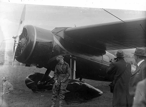
Figure: The Little Red Bus, Amelia Earhart’s plane in Derry after landing.

Earhart had navigated initially by dead reckoning and then through vision. Her hand was directly connected to the control surfaces of her plane through a series of linkages and cables. She could literally feel the plane in flight, she could respond to it and her environment to control her direction and destiny.

See Lawrence (2024) Earhart, Amelia p. 200–205.

NACA Langley

The feel of an aircraft is a repeated theme in the early years of flight. In response to perceived European advances in flight in the First World War, the US introduced the National Advisory Committee on Aeronautics. Under the committee a proving ground for aircraft was formed at Langley Field in Virginia. During the Second World War Bob Gilruth published a report on the flying qualities of aircraft that characterised how this feel could be translated into numbers.

See Lawrence (2024) Gilruth, Bob p. 190-192.

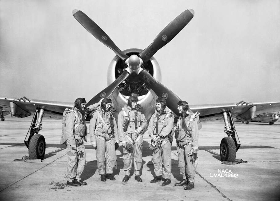
Figure: 1945 photo of the NACA test pilots, from left Mel Gough, Herb Hoover, Jack Reeder, Stefan Cavallo and Bill Gray (photo NASA, NACA LMAL 42612)

See Lawrence (2024) National Advisory Committee on Aeronautics (NACA) p. 163–168. One of Gilruth’s collaborators suggested that

Hawker Hurricane airplane. A heavily armed fighter airplane noted for its role in the Battle of Britain, the Hurricane’s flying qualities were found to be generally satisfactory. The most notable deficiencies were heavy aileron forces at high speeds and large friction in the controls.

W. Hewitt Phillips¹

and

Supermarine Spitfire airplane. A high-performance fighter noted for its role in the Battle of Britain and throughout WW II, the Spitfire had desirably light elevator control forces in maneuvers and near neutral longitudinal stability. Its greatest deficiency from the combat standpoint was heavy aileron forces and sluggish roll response at high speeds.

W. Hewitt Phillips²

Gilruth went beyond the reports of feel to characterise how the plane should respond to different inputs on the control stick. In other words he quantified that feel of the plane.

Gilrtuth’s work was in the spirit of Lord Kelvin’s quote on measurement

When you can measure what you are speaking about, and express it in numbers, you know something about it, when you cannot express it in numbers, your knowledge is of a meager and unsatisfactory kind; it may be the beginning of knowledge, but you have scarely, in your thoughts advanced to the stage of science.

From Chapter 3, pg 73 of Thomson (1889)

The aim was to convert a qualitative property of aircraft into quantitative measurement, thereby allowing their improvement.

The Atomic Human

Figure: The Atomic Eye, by slicing away aspects of the human that we used to believe to be unique to us, but are now the preserve of the machine, we learn something about what it means to be human.

The development of what some are calling intelligence in machines, raises questions around what machine intelligence means for our intelligence. The idea of the atomic human is derived from Democritus’s atomism.

In the fifth century bce the Greek philosopher Democritus posed a similar question about our physical universe. He imagined cutting physical matter into pieces in a repeated process: cutting a piece, then taking one of the cut pieces and cutting it again so that each time it becomes smaller and smaller. Democritus believed this process had to stop somewhere, that we would be left with an indivisible piece. The Greek word for indivisible is atom, and so this theory was called atomism. This book considers this question, but in a different domain, asking: As the machine slices away portions of human capabilities, are we left with a kernel of humanity, an indivisible piece that can no longer be divided into parts? Or does the human disappear altogether? If we are left with something, then that uncuttable piece, a form of atomic human, would tell us something about our human spirit.

See Lawrence (2024) atomic human, the p. 13.

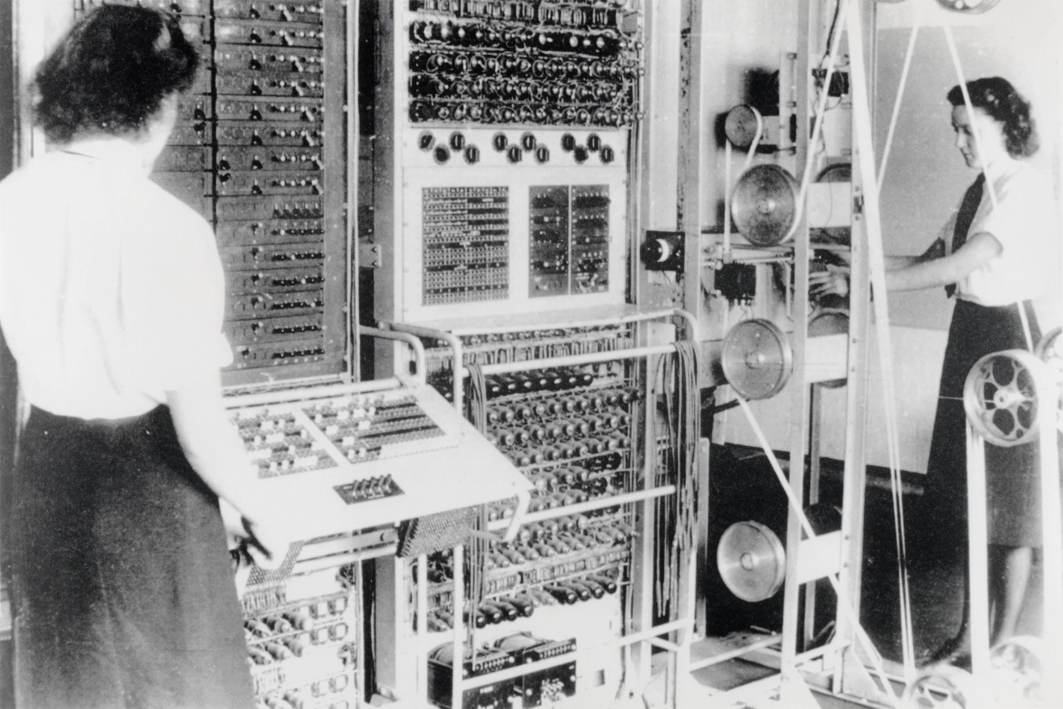
Figure: A Colossus Mark II codebreaking computer being operated by Dorothy Du Boisson (left) and Elsie Booker (right). Colossus was designed by Tommy Flowers, but programmed and operated by groups of Wrens based at Bletchley Park.

In the early hours of 1 June 1944, Tommy Flowers was wading ankle deep in water from a broken pipe, making the final connections to bring Mark 2 Colossus online. Colossus was the world’s first programmable, electronic, digital computer. Four days later, and Eisenhower was reading one of its first decrypts and ordering the invasion of Normandy. Flowers’s machine didn’t just launch an invasion, it launched an intellectual revolution.

See Lawrence (2024) Colossus (computer) p. 76–79, 91, 103, 108, 124, 130, 142–143, 149, 173–176, 199, 231–232, 251, 264, 267, 290, 380.

Embodiment Factors

bits/min	billions	2,000
billion calculations/s	~100	a billion
embodiment	20 minutes	5 billion years

Figure: Embodiment factors are the ratio between our ability to compute and our ability to communicate. Relative to the machine we are also locked in. In the table we represent embodiment as the length of time it would take to communicate one second’s worth of computation. For computers it is a matter of minutes, but for a human, it is a matter of thousands of millions of years. See also “Living Together: Mind and Machine Intelligence” Lawrence (2017)

There is a fundamental limit placed on our intelligence based on our ability to communicate. Claude Shannon founded the field of information theory. The clever part of this theory is it allows us to separate our measurement of information from what the information pertains to.³

Shannon measured information in bits. One bit of information is the amount of information I pass to you when I give you the result of a coin toss. Shannon was also interested in the amount of information in the English language. He estimated that on average a word in the English language contains 12 bits of information.

Given typical speaking rates, that gives us an estimate of our ability to communicate of around 100 bits per second (Reed and Durlach, 1998). Computers on the other hand can communicate much more rapidly. Current wired network speeds are around a billion bits per second, ten million times faster.

When it comes to compute though, our best estimates indicate our computers are slower. A typical modern computer can process make around 100 billion floating-point operations per second, each floating-point operation involves a 64 bit number. So the computer is processing around 6,400 billion bits per second.

It’s difficult to get similar estimates for humans, but by some estimates the amount of compute we would require to simulate a human brain is equivalent to that in the UK’s fastest computer (Ananthanarayanan et al., 2009), the MET office machine in Exeter, which in 2018 ranked as the 11th fastest computer in the world. That machine simulates the world’s weather each morning, and then simulates the world’s climate in the afternoon. It is a 16-petaflop machine, processing around 1,000 trillion bits per second.

See Lawrence (2024) embodiment factor p. 13, 29, 35, 79, 87, 105, 197, 216-217, 249, 269, 353, 369.

New Flow of Information

Classically the field of statistics focused on mediating the relationship between the machine and the human. Our limited bandwidth of communication means we tend to over-interpret the limited information that we are given, in the extreme we assign motives and desires to inanimate objects (a process known as anthropomorphizing). Much of mathematical statistics was developed to help temper this tendency and understand when we are valid in drawing conclusions from data.

Figure: The trinity of human, data, and computer, and highlights the modern phenomenon. The communication channel between computer and data now has an extremely high bandwidth. The channel between human and computer and the channel between data and human is narrow. New direction of information flow, information is reaching us mediated by the computer. The focus on classical statistics reflected the importance of the direct communication between human and data. The modern challenges of data science emerge when that relationship is being mediated by the machine.

Data science brings new challenges. In particular, there is a very large bandwidth connection between the machine and data. This means that our relationship with data is now commonly being mediated by the machine. Whether this is in the acquisition of new data, which now happens by happenstance rather than with purpose, or the interpretation of that data where we are increasingly relying on machines to summarize what the data contains. This is leading to the emerging field of data science, which must not only deal with the same challenges that mathematical statistics faced in tempering our tendency to over interpret data but must also deal with the possibility that the machine has either inadvertently or maliciously misrepresented the underlying data.

Fast Intelligence

Braitenberg Vehicles

Figure: Valentino Braitenberg was interested in synthetic psychology, he considered simple vehicles that react to their environment.

See Lawrence (2024) Braitenberg Vehicles p. 128-133, 143, 144, 146, 147-148.

Donald MacKay

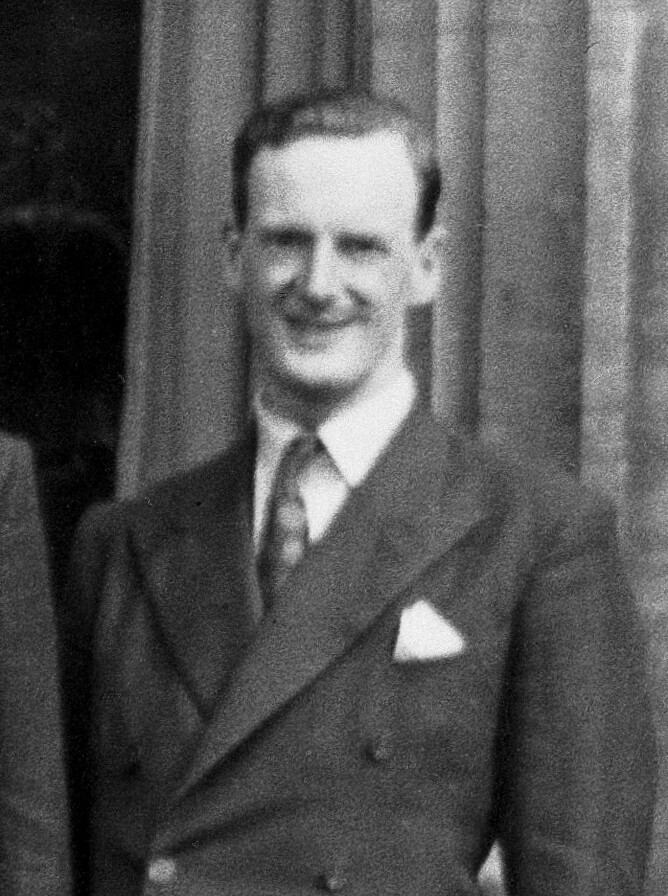
Figure: Donald M. MacKay (1922-1987), a physicist who was an early member of the cybernetics community and member of the Ratio Club.

Donald MacKay was a physicist who worked on naval gun targetting during the second world war. The challenge with gun targetting for ships is that both the target and the gun platform are moving. The challenge was tackled using analogue computers, for example in the US the Mark I fire control computer which was a mechanical computer. MacKay worked on radar systems for gun laying, here the velocity and distance of the target could be assessed through radar and an mechanical electrical analogue computer.

Fire Control Systems

Naval gunnery systems deal with targeting guns while taking into account movement of ships. The Royal Navy’s Gunnery Pocket Book (The Admiralty, 1945) gives details of one system for gun laying.

Like many challenges we face today, in the second world war, fire control was handled by a hybrid system of humans and computers. This means deploying human beings for the tasks that they can manage, and machines for the tasks that are better performed by a machine. This leads to a division of labour between the machine and the human that can still be found in our modern digital ecosystems.

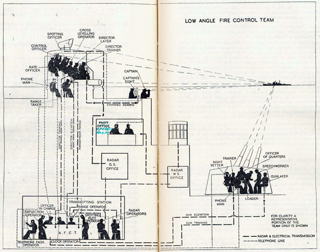
Figure: The fire control computer set at the centre of a system of observation and tracking (The Admiralty, 1945).

As analogue computers, fire control computers from the second world war would contain components that directly represented the different variables that were important in the problem to be solved, such as the inclination between two ships.

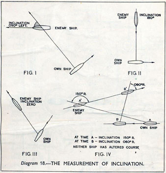
Figure: Measuring inclination between two ships (The Admiralty, 1945). Sophisticated fire control computers allowed the ship to continue to fire while under maneuvers.

The fire control systems were electro-mechanical analogue computers that represented the “state variables” of interest, such as inclination and ship speed with gears and cams within the machine.

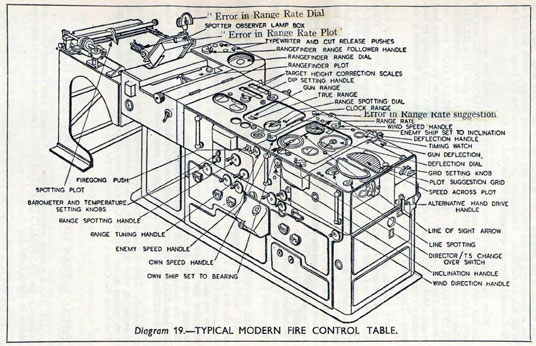
Figure: A second world war gun computer’s control table (The Admiralty, 1945).

For more details on fire control computers, you can watch a 1953 film on the the US the Mark IA fire control computer from Periscope Film.

Figure: U.S. Navy training film MN-6783a. Basic Mechanisms of Fire Control Computers. Mechanical Computer Instructional Film 27794 (1953) for the Mk 1A Fire Control Computer.

Behind the Eye

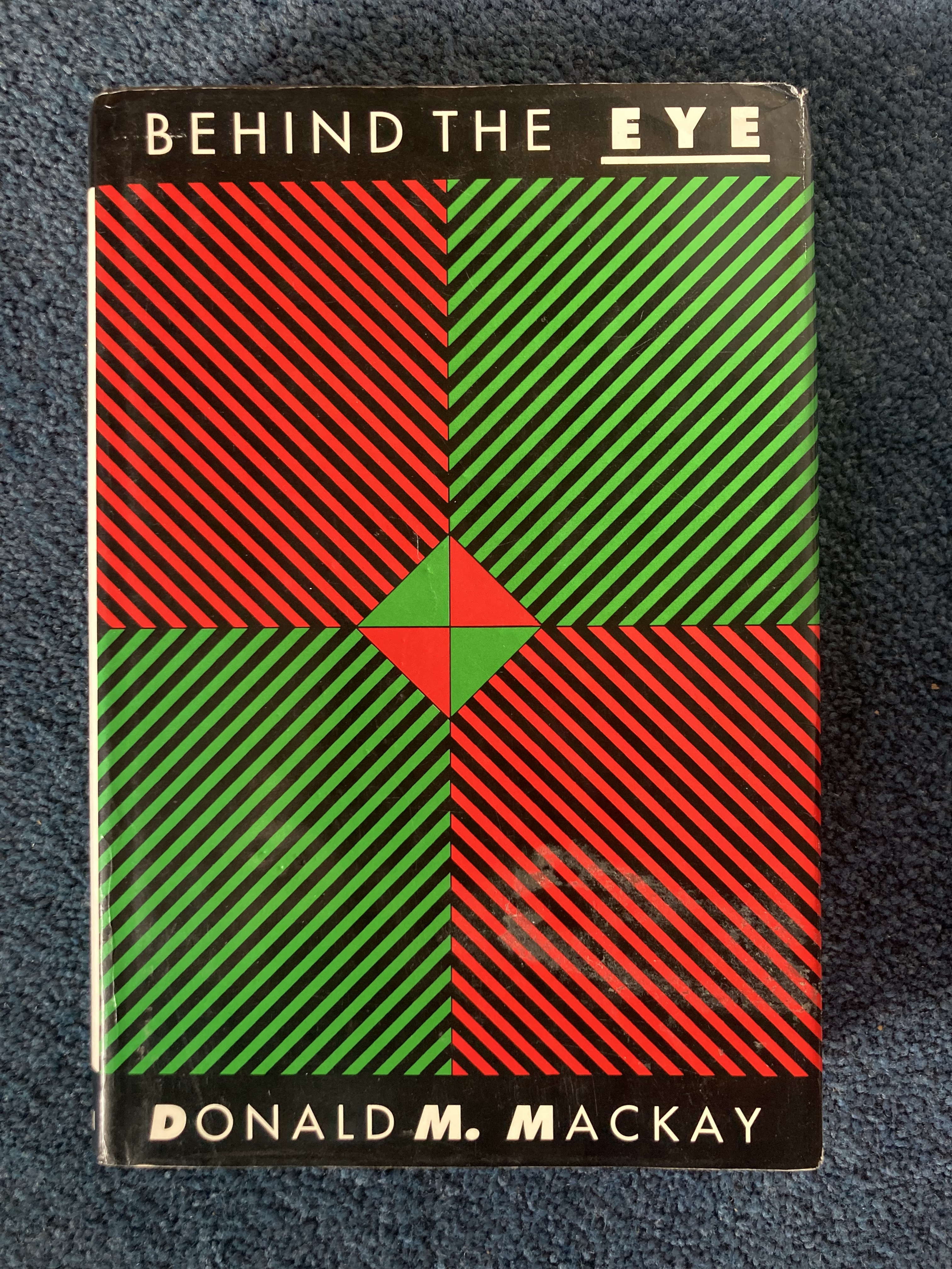
Figure: Behind the Eye (MacKay, 1991) summarises MacKay’s Gifford Lectures, where MacKay uses the operation of the eye as a window on the operation of the brain.

Donald MacKay was at King’s College for his PhD. He was just down the road from Bill Phillips at LSE who was building the MONIAC. He was part of the Ratio Club. A group of early career scientists who were interested in communication and control in animals and humans, or more specifically they were interested in computers and brains. The were part of an international movement known as cybernetics.

Donald MacKay wrote of the influence that his own work on radar had on his interest in the brain.

… during the war I had worked on the theory of automated and electronic computing and on the theory of information, all of which are highly relevant to such things as automatic pilots and automatic gun direction. I found myself grappling with problems in the design of artificial sense organs for naval gun-directors and with the principles on which electronic circuits could be used to simulate situations in the external world so as to provide goal-directed guidance for ships, aircraft, missiles and the like.

Later in the 1940’s, when I was doing my Ph.D. work, there was much talk of the brain as a computer and of the early digital computers that were just making the headlines as “electronic brains.” As an analogue computer man I felt strongly convinced that the brain, whatever it was, was not a digital computer. I didn’t think it was an analogue computer either in the conventional sense.

But this naturally rubbed under my skin the question: well, if it is not either of these, what kind of system is it? Is there any way of following through the kind of analysis that is appropriate to their artificial automata so as to understand better the kind of system the human brain is? That was the beginning of my slippery slope into brain research.

Behind the Eye pg 40. Edited version of the 1986 Gifford Lectures given by Donald M. MacKay and edited by Valerie MacKay

See Lawrence (2024) MacKay, Donald, Behind the Eye p. 268-270, 316.

Importantly, MacKay distinguishes between the analogue computer and the digital computer. As he mentions, his experience was with analogue machines. An analogue machine is literally an analogue. The radar systems that Wiener and MacKay both worked on were made up of electronic components such as resistors, capacitors, inductors and/or mechanical components such as cams and gears. Together these components could represent a physical system, such as an anti-aircraft gun and a plane. The design of the analogue computer required the engineer to simulate the real world in analogue electronics, using dualities that exist between e.g. mechanical circuits (mass, spring, damper) and electronic circuits (inductor, resistor, capacitor). The analogy between mass and a damper, between spring and a resistor and between capacitor and a damper works because the underlying mathematics is approximated with the same linear system: a second order differential equation. This mathematical analogy allowed the designer to map from the real world, through mathematics, to a virtual world where the components reflected the real world through analogy.

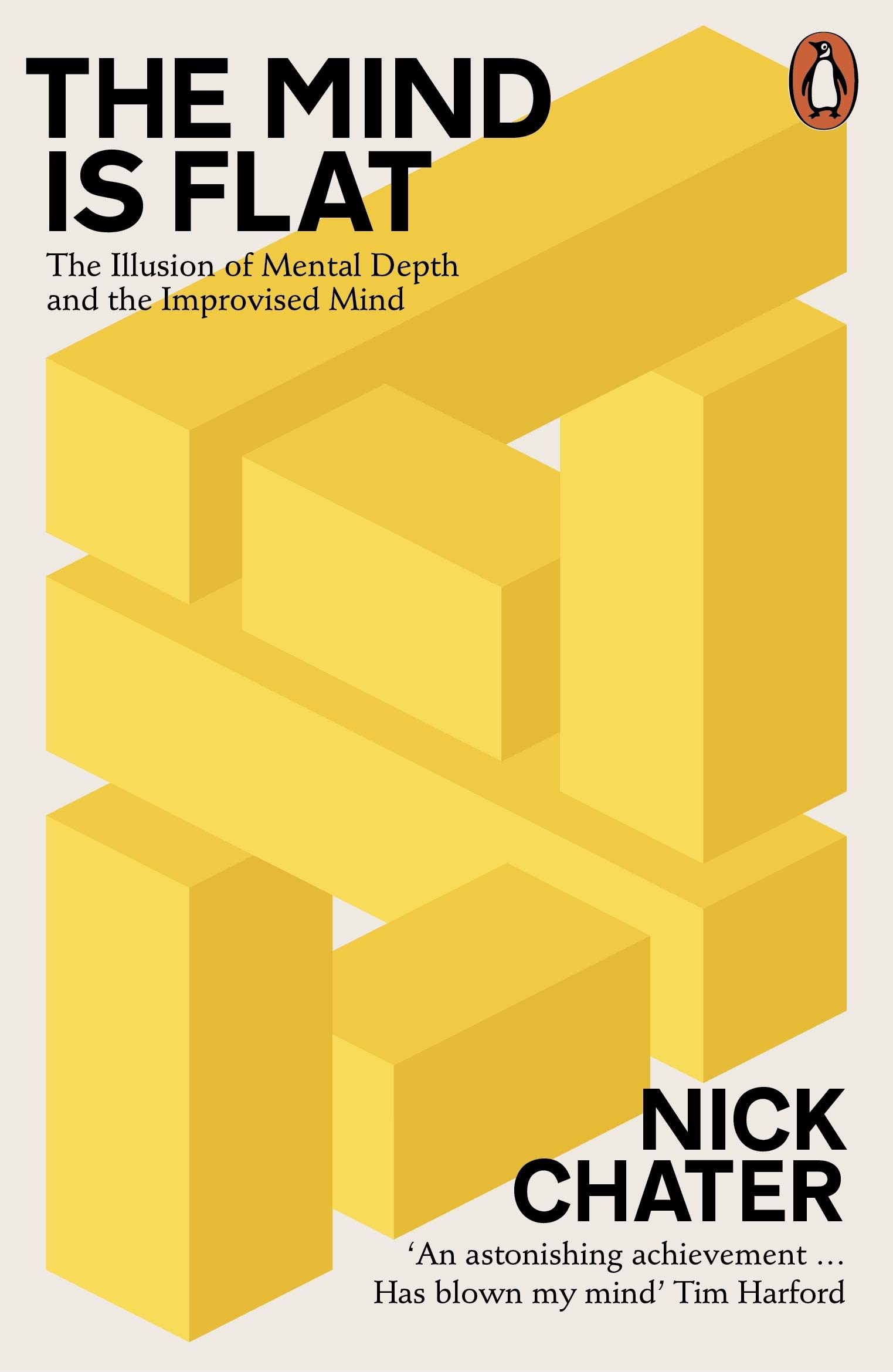
Figure: The Mind is Flat Nick Chater relates the extent to which how we are is determined by the data we see.

(Chater, 2019)

Slow Intelligence

}

Figure: Behind the Mirror (Lorenz, 1977) introduces the notion of thinking as acting in an imagined space. (see also work by Bernhard Schölkopf.

(Lorenz, 1977)

Elohim Creating Adam

Blake’s vision of the creation of man, known as Elohim Creating Adam, is a strong contrast to Michelangelo’s. The faces of both God and Adam show deep anguish. The image is closer to representations of Prometheus receiving his punishment for sharing his knowledge of fire than to the languid ecstasy we see in Michelangelo’s representation.

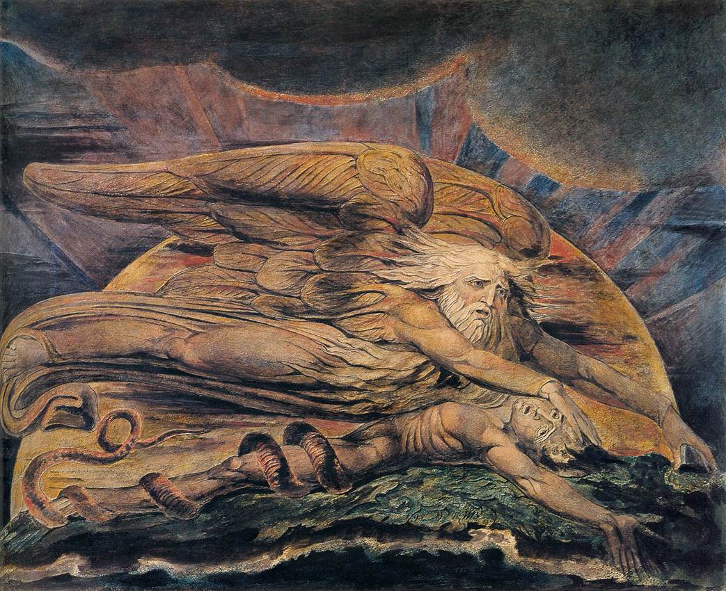
Figure: William Blake’s Elohim Creating Adam.

The caption in the Tate reads:

Elohim is a Hebrew name for God. This picture illustrates the Book of Genesis: ‘And the Lord God formed man of the dust of the ground’. Adam is shown growing out of the earth, a piece of which Elohim holds in his left hand.

For Blake the God of the Old Testament was a false god. He believed the Fall of Man took place not in the Garden of Eden, but at the time of creation shown here, when man was dragged from the spiritual realm and made material.

From the Tate Britain

Blake’s vision is demonstrating the frustrations we experience when the (complex) real world doesn’t manifest in the way we’d hoped.

See Lawrence (2024) Blake, William Elohim Creating Adam p. 121, 217–18.

Human Analogue Machine

Recent breakthroughs in generative models, particularly large language models, have enabled machines that, for the first time, can converse plausibly with other humans.

The Apollo guidance computer provided Armstrong with an analogy when he landed it on the Moon. He controlled it through a stick which provided him with an analogy. The analogy is based in the experience that Amelia Earhart had when she flew her plane. Armstrong’s control exploited his experience as a test pilot flying planes that had control columns which were directly connected to their control surfaces.

Figure:

The generative systems we have produced do not provide us with the “AI” of science fiction. Because their intelligence is based on emulating human knowledge. Through being forced to reproduce our literature and our art they have developed aspects which are analogous to the cultural proxy truths we use to describe our world.

These machines are to humans what the MONIAC was the British economy. Not a replacement, but an analogue computer that captures some aspects of humanity while providing advantages of high bandwidth of the machine.

HAM

The Human-Analogue Machine or HAM therefore provides a route through which we could better understand our world through improving the way we interact with machines.

Figure: The trinity of human, data, and computer, and highlights the modern phenomenon. The communication channel between computer and data now has an extremely high bandwidth. The channel between human and computer and the channel between data and human is narrow. New direction of information flow, information is reaching us mediated by the computer. The focus on classical statistics reflected the importance of the direct communication between human and data. The modern challenges of data science emerge when that relationship is being mediated by the machine.

The HAM can provide an interface between the digital computer and the human allowing humans to work closely with computers regardless of their understandin gf the more technical parts of software engineering.

Figure: The HAM now sits between us and the traditional digital computer.

Of course this route provides new routes for manipulation, new ways in which the machine can undermine our autonomy or exploit our cognitive foibles. The major challenge we face is steering between these worlds where we gain the advantage of the computer’s bandwidth without undermining our culture and individual autonomy.

See Lawrence (2024) human-analogue machine (HAMs) p. 343-347, 359-359, 365-368.

Atrophy and Cognitive Flattening

Even if we calibrate these tools correctly so that they do represent the world appropriately we are at risk. The hippocampus is part of our brain’s cortex, oOne role of our hippocampus is in navigation, knowing how to move from one place to another.

Figure: The hippocampus within the brain. Image generated from Anatomography, https://lifesciencedb.jp/.

Our prefrontal cortex, the size of which differentiates us from other primates and mammals, is the seat of our planning and of our higher intelligence. It fires in sympathy with our hippocampus.

Figure: Navigation is helpful but we can become overreliant on it. News article from people.com.

By becoming overreliant on HAMs and there interface to the digital computer are we at risk of suffering from the same deskilling we perceive in our navigational skills? Does this place us at risk of sleepwalking into a world that is managed by the machine even as we believe that we are managing it ourselves?

The Atomic Human

Figure: The Atomic Human (Lawrence, 2024).

Thanks!

For more information on these subjects and more you might want to check the following resources.

• book: The Atomic Human
• twitter: @lawrennd
• podcast: The Talking Machines
• newspaper: Guardian Profile Page
• blog: http://inverseprobability.com

References