Abstract

What if machines could think like humans? Can AI truly understand us? Ever wondered how AI will shape our future?

Discover some of the answers with Neil Lawrence, one of the world’s foremost experts in AI and machine learning. In this insightful talk, Neil Lawrence will reveal how AI serves as a powerful assistant to human intelligence, not a replacement. He will discuss the limits of AI in replicating human thought and its profound impact on society and information management.

Additionally, the talk will explore our society’s fascination and fears about AI, examining its influence on human identity. Lawrence will give an overview of the current state of AI, the challenges we face, and the importance of transparency and data quality. This session will offer valuable insights into the real-world applications of AI and its future.

Neil Lawrence is the inaugural DeepMind Professor of Machine Learning at the University of Cambridge where he is also the academic lead of AI@Cam, the University’s flagship mission on AI. He has been working on machine learning models for over 25 years. He returned to academia in 2019 after three years as Director of Machine Learning at Amazon. He is also a Senior AI Fellow at the Alan Turing Institute, visiting Professor at the University of Sheffield and author of the book The Atomic Human - understanding ourselves in the age of AI.

Henry Ford’s Faster Horse

Figure: A 1925 Ford Model T built at Henry Ford’s Highland Park Plant in Dearborn, Michigan. This example now resides in Australia, owned by the founder of FordModelT.net. From https://commons.wikimedia.org/wiki/File:1925_Ford_Model_T_touring.jpg

It’s said that Henry Ford’s customers wanted a “a faster horse”. If Henry Ford was selling us artificial intelligence today, what would the customer call for, “a smarter human”? That’s certainly the picture of machine intelligence we find in science fiction narratives, but the reality of what we’ve developed is much more mundane.

Car engines produce prodigious power from petrol. Machine intelligences deliver decisions derived from data. In both cases the scale of consumption enables a speed of operation that is far beyond the capabilities of their natural counterparts. Unfettered energy consumption has consequences in the form of climate change. Does unbridled data consumption also have consequences for us?

If we devolve decision making to machines, we depend on those machines to accommodate our needs. If we don’t understand how those machines operate, we lose control over our destiny. Our mistake has been to see machine intelligence as a reflection of our intelligence. We cannot understand the smarter human without understanding the human. To understand the machine, we need to better understand ourselves.

The Atomic Human

Figure: The Atomic Eye, by slicing away aspects of the human that we used to believe to be unique to us, but are now the preserve of the machine, we learn something about what it means to be human.

The development of what some are calling intelligence in machines, raises questions around what machine intelligence means for our intelligence. The idea of the atomic human is derived from Democritus’s atomism.

In the fifth century bce the Greek philosopher Democritus posed a similar question about our physical universe. He imagined cutting physical matter into pieces in a repeated process: cutting a piece, then taking one of the cut pieces and cutting it again so that each time it becomes smaller and smaller. Democritus believed this process had to stop somewhere, that we would be left with an indivisible piece. The Greek word for indivisible is atom, and so this theory was called atomism. This book considers this question, but in a different domain, asking: As the machine slices away portions of human capabilities, are we left with a kernel of humanity, an indivisible piece that can no longer be divided into parts? Or does the human disappear altogether? If we are left with something, then that uncuttable piece, a form of atomic human, would tell us something about our human spirit.

See Lawrence (2024) atomic human, the p. 13.

The Diving Bell and the Butterfly

Figure: The Diving Bell and the Buttefly is the autobiography of Jean Dominique Bauby.

The Diving Bell and the Butterfly is the autobiography of Jean Dominique Bauby. Jean Dominique, the editor of French Elle magazine, suffered a major stroke at the age of 43 in 1995. The stroke paralyzed him and rendered him speechless. He was only able to blink his left eyelid, he became a sufferer of locked in syndrome.

See Lawrence (2024) Le Scaphandre et le papillon (The Diving Bell and the Butterfly) p. 10–12.

E S A R I N T U L
O M D P C F B V
H G J Q Z Y X K W

Figure: The ordering of the letters that Bauby used for writing his autobiography.

How could he do that? Well, first, they set up a mechanism where he could scan across letters and blink at the letter he wanted to use. In this way, he was able to write each letter.

It took him 10 months of four hours a day to write the book. Each word took two minutes to write.

Imagine doing all that thinking, but so little speaking, having all those thoughts and so little ability to communicate.

One challenge for the atomic human is that we are all in that situation. While not as extreme as for Bauby, when we compare ourselves to the machine, we all have a locked-in intelligence.

Figure: Jean Dominique Bauby was the Editor in Chief of the French Elle Magazine, he suffered a stroke that destroyed his brainstem, leaving him only capable of moving one eye. Jean Dominique became a victim of locked in syndrome.

Incredibly, Jean Dominique wrote his book after he became locked in. It took him 10 months of four hours a day to write the book. Each word took two minutes to write.

The idea behind embodiment factors is that we are all in that situation. While not as extreme as for Bauby, we all have somewhat of a locked in intelligence.

See Lawrence (2024) Bauby, Jean Dominique p. 9–11, 18, 90, 99-101, 133, 186, 212–218, 234, 240, 251–257, 318, 368–369.

Bauby and Shannon

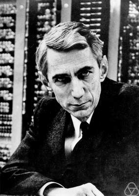
Figure: Claude Shannon developed information theory which allows us to quantify how much Bauby can communicate. This allows us to compare how locked in he is to us.

See Lawrence (2024) Shannon, Claude p. 10, 30, 61, 74, 98, 126, 134, 140, 143, 149, 260, 264, 269, 277, 315, 358, 363.

Embodiment Factors

bits/min	billions	2000	6
billion calculations/s	~100	a billion	a billion
embodiment	20 minutes	5 billion years	15 trillion years

Figure: Embodiment factors are the ratio between our ability to compute and our ability to communicate. Jean Dominique Bauby suffered from locked-in syndrome. The embodiment factors show that relative to the machine we are also locked in. In the table we represent embodiment as the length of time it would take to communicate one second’s worth of computation. For computers it is a matter of minutes, but for a human, whether locked in or not, it is a matter of many millions of years.

Let me explain what I mean. Claude Shannon introduced a mathematical concept of information for the purposes of understanding telephone exchanges.

Information has many meanings, but mathematically, Shannon defined a bit of information to be the amount of information you get from tossing a coin.

If I toss a coin, and look at it, I know the answer. You don’t. But if I now tell you the answer I communicate to you 1 bit of information. Shannon defined this as the fundamental unit of information.

If I toss the coin twice, and tell you the result of both tosses, I give you two bits of information. Information is additive.

Shannon also estimated the average information associated with the English language. He estimated that the average information in any word is 12 bits, equivalent to twelve coin tosses.

So every two minutes Bauby was able to communicate 12 bits, or six bits per minute.

This is the information transfer rate he was limited to, the rate at which he could communicate.

Compare this to me, talking now. The average speaker for TEDX speaks around 160 words per minute. That’s 320 times faster than Bauby or around a 2000 bits per minute. 2000 coin tosses per minute.

But, just think how much thought Bauby was putting into every sentence. Imagine how carefully chosen each of his words was. Because he was communication constrained he could put more thought into each of his words. Into thinking about his audience.

So, his intelligence became locked in. He thinks as fast as any of us, but can communicate slower. Like the tree falling in the woods with no one there to hear it, his intelligence is embedded inside him.

Two thousand coin tosses per minute sounds pretty impressive, but this talk is not just about us, it’s about our computers, and the type of intelligence we are creating within them.

So how does two thousand compare to our digital companions? When computers talk to each other, they do so with billions of coin tosses per minute.

Let’s imagine for a moment, that instead of talking about communication of information, we are actually talking about money. Bauby would have 6 dollars. I would have 2000 dollars, and my computer has billions of dollars.

The internet has interconnected computers and equipped them with extremely high transfer rates.

However, by our very best estimates, computers actually think slower than us.

How can that be? You might ask, computers calculate much faster than me. That’s true, but underlying your conscious thoughts there are a lot of calculations going on.

Each thought involves many thousands, millions or billions of calculations. How many exactly, we don’t know yet, because we don’t know how the brain turns calculations into thoughts.

Our best estimates suggest that to simulate your brain a computer would have to be as large as the UK Met Office machine here in Exeter. That’s a 250 million pound machine, the fastest in the UK. It can do 16 billion billon calculations per second.

It simulates the weather across the word every day, that’s how much power we think we need to simulate our brains.

So, in terms of our computational power we are extraordinary, but in terms of our ability to explain ourselves, just like Bauby, we are locked in.

For a typical computer, to communicate everything it computes in one second, it would only take it a couple of minutes. For us to do the same would take 15 billion years.

If intelligence is fundamentally about processing and sharing of information. This gives us a fundamental constraint on human intelligence that dictates its nature.

I call this ratio between the time it takes to compute something, and the time it takes to say it, the embodiment factor (Lawrence, 2017). Because it reflects how embodied our cognition is.

If it takes you two minutes to say the thing you have thought in a second, then you are a computer. If it takes you 15 billion years, then you are a human.

Bandwidth Constrained Conversations

Figure: Conversation relies on internal models of other individuals.

Figure: Misunderstanding of context and who we are talking to leads to arguments.

Embodiment factors imply that, in our communication between humans, what is not said is, perhaps, more important than what is said. To communicate with each other we need to have a model of who each of us are.

To aid this, in society, we are required to perform roles. Whether as a parent, a teacher, an employee or a boss. Each of these roles requires that we conform to certain standards of behaviour to facilitate communication between ourselves.

Control of self is vitally important to these communications.

The high availability of data available to humans undermines human-to-human communication channels by providing new routes to undermining our control of self.

The consequences between this mismatch of power and delivery are to be seen all around us. Because, just as driving an F1 car with bicycle wheels would be a fine art, so is the process of communication between humans.

If I have a thought and I wish to communicate it, I first need to have a model of what you think. I should think before I speak. When I speak, you may react. You have a model of who I am and what I was trying to say, and why I chose to say what I said. Now we begin this dance, where we are each trying to better understand each other and what we are saying. When it works, it is beautiful, but when mis-deployed, just like a badly driven F1 car, there is a horrible crash, an argument.

Computer Conversations

Figure: Conversation relies on internal models of other individuals.

Figure: Misunderstanding of context and who we are talking to leads to arguments.

Similarly, we find it difficult to comprehend how computers are making decisions. Because they do so with more data than we can possibly imagine.

In many respects, this is not a problem, it’s a good thing. Computers and us are good at different things. But when we interact with a computer, when it acts in a different way to us, we need to remember why.

Just as the first step to getting along with other humans is understanding other humans, so it needs to be with getting along with our computers.

Embodiment factors explain why, at the same time, computers are so impressive in simulating our weather, but so poor at predicting our moods. Our complexity is greater than that of our weather, and each of us is tuned to read and respond to one another.

Their intelligence is different. It is based on very large quantities of data that we cannot absorb. Our computers don’t have a complex internal model of who we are. They don’t understand the human condition. They are not tuned to respond to us as we are to each other.

Embodiment factors encapsulate a profound thing about the nature of humans. Our locked in intelligence means that we are striving to communicate, so we put a lot of thought into what we’re communicating with. And if we’re communicating with something complex, we naturally anthropomorphize them.

We give our dogs, our cats, and our cars human motivations. We do the same with our computers. We anthropomorphize them. We assume that they have the same objectives as us and the same constraints. They don’t.

This means, that when we worry about artificial intelligence, we worry about the wrong things. We fear computers that behave like more powerful versions of ourselves that will struggle to outcompete us.

In reality, the challenge is that our computers cannot be human enough. They cannot understand us with the depth we understand one another. They drop below our cognitive radar and operate outside our mental models.

The real danger is that computers don’t anthropomorphize. They’ll make decisions in isolation from us without our supervision because they can’t communicate truly and deeply with us.

New Flow of Information

Classically the field of statistics focused on mediating the relationship between the machine and the human. Our limited bandwidth of communication means we tend to over-interpret the limited information that we are given, in the extreme we assign motives and desires to inanimate objects (a process known as anthropomorphizing). Much of mathematical statistics was developed to help temper this tendency and understand when we are valid in drawing conclusions from data.

Figure: The trinity of human, data, and computer, and highlights the modern phenomenon. The communication channel between computer and data now has an extremely high bandwidth. The channel between human and computer and the channel between data and human is narrow. New direction of information flow, information is reaching us mediated by the computer. The focus on classical statistics reflected the importance of the direct communication between human and data. The modern challenges of data science emerge when that relationship is being mediated by the machine.

Data science brings new challenges. In particular, there is a very large bandwidth connection between the machine and data. This means that our relationship with data is now commonly being mediated by the machine. Whether this is in the acquisition of new data, which now happens by happenstance rather than with purpose, or the interpretation of that data where we are increasingly relying on machines to summarize what the data contains. This is leading to the emerging field of data science, which must not only deal with the same challenges that mathematical statistics faced in tempering our tendency to over interpret data but must also deal with the possibility that the machine has either inadvertently or maliciously misrepresented the underlying data.

A Six Word Novel

Figure: Consider the six-word novel, apocryphally credited to Ernest Hemingway, “For sale: baby shoes, never worn”. To understand what that means to a human, you need a great deal of additional context. Context that is not directly accessible to a machine that has not got both the evolved and contextual understanding of our own condition to realize both the implication of the advert and what that implication means emotionally to the previous owner.

See Lawrence (2024) baby shoes p. 368.

But this is a very different kind of intelligence than ours. A computer cannot understand the depth of the Ernest Hemingway’s apocryphal six-word novel: “For Sale, Baby Shoes, Never worn”, because it isn’t equipped with that ability to model the complexity of humanity that underlies that statement.

Blake’s Newton

William Blake’s rendering of Newton captures humans in a particular state. He is trance-like absorbed in simple geometric shapes. The feel of dreams is enhanced by the underwater location, and the nature of the focus is enhanced because he ignores the complexity of the sea life around him.

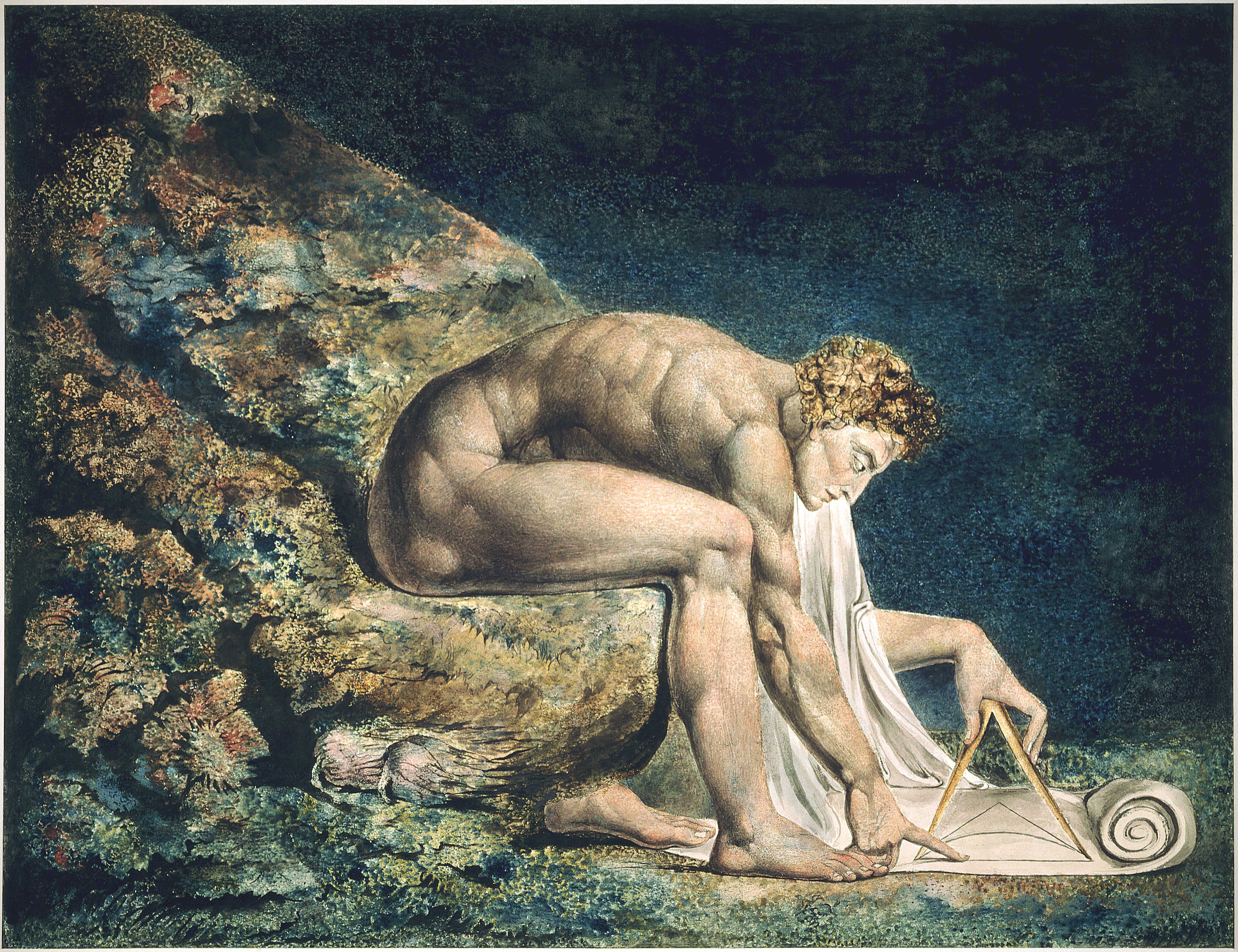
Figure: William Blake’s Newton. 1795c-1805

See Lawrence (2024) Blake, William Newton p. 121–123.

The caption in teh Tate Britain reads:

Here, Blake satirises the 17th-century mathematician Isaac Newton. Portrayed as a muscular youth, Newton seems to be underwater, sitting on a rock covered with colourful coral and lichen. He crouches over a diagram, measuring it with a compass. Blake believed that Newton’s scientific approach to the world was too reductive. Here he implies Newton is so fixated on his calculations that he is blind to the world around him. This is one of only 12 large colour prints Blake made. He seems to have used an experimental hybrid of printing, drawing, and painting.

From the Tate Britain

See Lawrence (2024) Blake, William Newton p. 121–123, 258, 260, 283, 284, 301, 306.

The MONIAC

The MONIAC was an analogue computer designed to simulate the UK economy. Analogue comptuers work through analogy, the analogy in the MONIAC is that both money and water flow. The MONIAC exploits this through a system of tanks, pipes, valves and floats that represent the flow of money through the UK economy. Water flowed from the treasury tank at the top of the model to other tanks representing government spending, such as health and education. The machine was initially designed for teaching support but was also found to be a useful economic simulator. Several were built and today you can see the original at Leeds Business School, there is also one in the London Science Museum and one in the Unisversity of Cambridge’s economics faculty.

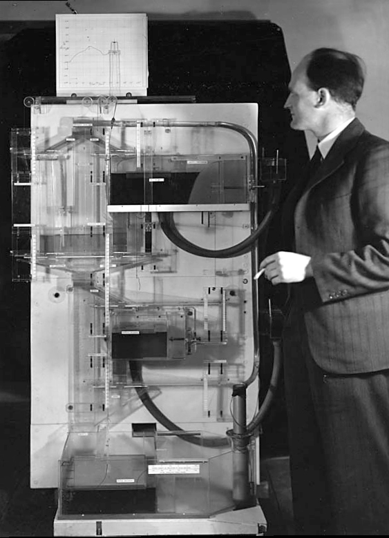
Figure: Bill Phillips and his MONIAC (completed in 1949). The machine is an analogue computer designed to simulate the workings of the UK economy.

See Lawrence (2024) MONIAC p. 232-233, 266, 343.

Human Analogue Machine

Recent breakthroughs in generative models, particularly large language models, have enabled machines that, for the first time, can converse plausibly with other humans.

The Apollo guidance computer provided Armstrong with an analogy when he landed it on the Moon. He controlled it through a stick which provided him with an analogy. The analogy is based in the experience that Amelia Earhart had when she flew her plane. Armstrong’s control exploited his experience as a test pilot flying planes that had control columns which were directly connected to their control surfaces.

Figure:

The generative systems we have produced do not provide us with the “AI” of science fiction. Because their intelligence is based on emulating human knowledge. Through being forced to reproduce our literature and our art they have developed aspects which are analogous to the cultural proxy truths we use to describe our world.

These machines are to humans what the MONIAC was the British economy. Not a replacement, but an analogue computer that captures some aspects of humanity while providing advantages of high bandwidth of the machine.

HAM

The Human-Analogue Machine or HAM therefore provides a route through which we could better understand our world through improving the way we interact with machines.

Figure: The trinity of human, data, and computer, and highlights the modern phenomenon. The communication channel between computer and data now has an extremely high bandwidth. The channel between human and computer and the channel between data and human is narrow. New direction of information flow, information is reaching us mediated by the computer. The focus on classical statistics reflected the importance of the direct communication between human and data. The modern challenges of data science emerge when that relationship is being mediated by the machine.

The HAM can provide an interface between the digital computer and the human allowing humans to work closely with computers regardless of their understandin gf the more technical parts of software engineering.

Figure: The HAM now sits between us and the traditional digital computer.

Of course this route provides new routes for manipulation, new ways in which the machine can undermine our autonomy or exploit our cognitive foibles. The major challenge we face is steering between these worlds where we gain the advantage of the computer’s bandwidth without undermining our culture and individual autonomy.

See Lawrence (2024) human-analogue machine (HAMs) p. 343-347, 359-359, 365-368.

Bandwidth vs Complexity

The computer communicates in Gigabits per second, One way of imagining just how much slower we are than the machine is to look for something that communicates in nanobits per second.

bits/min	\(100 \times 10^{-9}\)	\(2,000\)	\(600 \times 10^9\)

Figure: When we look at communication rates based on the information passing from one human to another across generations through their genetics, we see that computers watching us communicate is roughly equivalent to us watching organisms evolve. Estimates of germline mutation rates taken from Scally (2016).

Figure: Bandwidth vs Complexity.

The challenge we face is that while speed is on the side of the machine, complexity is on the side of our ecology. Many of the risks we face are associated with the way our speed undermines our ecology and the machines speed undermines our human culture.

See Lawrence (2024) Human evolution rates p. 98-99. See Lawrence (2024) Psychological representation of Ecologies p. 323-327.

Thanks!

For more information on these subjects and more you might want to check the following resources.

• book: The Atomic Human
• twitter: @lawrennd
• podcast: The Talking Machines
• newspaper: Guardian Profile Page
• blog: http://inverseprobability.com

References