edit

Caught by Surprise Retrospective: The Mechanistic Fallacy and Modelling How We Think

$$\newcommand{\tk}[1]{} \newcommand{\Amatrix}{\mathbf{A}} \newcommand{\KL}[2]{\text{KL}\left( #1\,\|\,#2 \right)} \newcommand{\Kaast}{\kernelMatrix_{\mathbf{ \ast}\mathbf{ \ast}}} \newcommand{\Kastu}{\kernelMatrix_{\mathbf{ \ast} \inducingVector}} \newcommand{\Kff}{\kernelMatrix_{\mappingFunctionVector \mappingFunctionVector}} \newcommand{\Kfu}{\kernelMatrix_{\mappingFunctionVector \inducingVector}} \newcommand{\Kuast}{\kernelMatrix_{\inducingVector \bf\ast}} \newcommand{\Kuf}{\kernelMatrix_{\inducingVector \mappingFunctionVector}} \newcommand{\Kuu}{\kernelMatrix_{\inducingVector \inducingVector}} \newcommand{\Kuui}{\Kuu^{-1}} \newcommand{\Qaast}{\mathbf{Q}_{\bf \ast \ast}} \newcommand{\Qastf}{\mathbf{Q}_{\ast \mappingFunction}} \newcommand{\Qfast}{\mathbf{Q}_{\mappingFunctionVector \bf \ast}} \newcommand{\Qff}{\mathbf{Q}_{\mappingFunctionVector \mappingFunctionVector}} \newcommand{\aMatrix}{\mathbf{A}} \newcommand{\aScalar}{a} \newcommand{\aVector}{\mathbf{a}} \newcommand{\acceleration}{a} \newcommand{\bMatrix}{\mathbf{B}} \newcommand{\bScalar}{b} \newcommand{\bVector}{\mathbf{b}} \newcommand{\basisFunc}{\phi} \newcommand{\basisFuncVector}{\boldsymbol{ \basisFunc}} \newcommand{\basisFunction}{\phi} \newcommand{\basisLocation}{\mu} \newcommand{\basisMatrix}{\boldsymbol{ \Phi}} \newcommand{\basisScalar}{\basisFunction} \newcommand{\basisVector}{\boldsymbol{ \basisFunction}} \newcommand{\activationFunction}{\phi} \newcommand{\activationMatrix}{\boldsymbol{ \Phi}} \newcommand{\activationScalar}{\basisFunction} \newcommand{\activationVector}{\boldsymbol{ \basisFunction}} \newcommand{\bigO}{\mathcal{O}} \newcommand{\binomProb}{\pi} \newcommand{\cMatrix}{\mathbf{C}} \newcommand{\cbasisMatrix}{\hat{\boldsymbol{ \Phi}}} \newcommand{\cdataMatrix}{\hat{\dataMatrix}} \newcommand{\cdataScalar}{\hat{\dataScalar}} \newcommand{\cdataVector}{\hat{\dataVector}} \newcommand{\centeredKernelMatrix}{\mathbf{ \MakeUppercase{\centeredKernelScalar}}} \newcommand{\centeredKernelScalar}{b} \newcommand{\centeredKernelVector}{\centeredKernelScalar} \newcommand{\centeringMatrix}{\mathbf{H}} \newcommand{\chiSquaredDist}[2]{\chi_{#1}^{2}\left(#2\right)} \newcommand{\chiSquaredSamp}[1]{\chi_{#1}^{2}} \newcommand{\conditionalCovariance}{\boldsymbol{ \Sigma}} \newcommand{\coregionalizationMatrix}{\mathbf{B}} \newcommand{\coregionalizationScalar}{b} \newcommand{\coregionalizationVector}{\mathbf{ \coregionalizationScalar}} \newcommand{\covDist}[2]{\text{cov}_{#2}\left(#1\right)} \newcommand{\covSamp}[1]{\text{cov}\left(#1\right)} \newcommand{\covarianceScalar}{c} \newcommand{\covarianceVector}{\mathbf{ \covarianceScalar}} \newcommand{\covarianceMatrix}{\mathbf{C}} \newcommand{\covarianceMatrixTwo}{\boldsymbol{ \Sigma}} \newcommand{\croupierScalar}{s} \newcommand{\croupierVector}{\mathbf{ \croupierScalar}} \newcommand{\croupierMatrix}{\mathbf{ \MakeUppercase{\croupierScalar}}} \newcommand{\dataDim}{p} \newcommand{\dataIndex}{i} \newcommand{\dataIndexTwo}{j} \newcommand{\dataMatrix}{\mathbf{Y}} \newcommand{\dataScalar}{y} \newcommand{\dataSet}{\mathcal{D}} \newcommand{\dataStd}{\sigma} \newcommand{\dataVector}{\mathbf{ \dataScalar}} \newcommand{\decayRate}{d} \newcommand{\degreeMatrix}{\mathbf{ \MakeUppercase{\degreeScalar}}} \newcommand{\degreeScalar}{d} \newcommand{\degreeVector}{\mathbf{ \degreeScalar}} \newcommand{\diag}[1]{\text{diag}\left(#1\right)} \newcommand{\diagonalMatrix}{\mathbf{D}} \newcommand{\diff}[2]{\frac{\text{d}#1}{\text{d}#2}} \newcommand{\diffTwo}[2]{\frac{\text{d}^2#1}{\text{d}#2^2}} \newcommand{\displacement}{x} \newcommand{\displacementVector}{\textbf{\displacement}} \newcommand{\distanceMatrix}{\mathbf{ \MakeUppercase{\distanceScalar}}} \newcommand{\distanceScalar}{d} \newcommand{\distanceVector}{\mathbf{ \distanceScalar}} \newcommand{\eigenvaltwo}{\ell} \newcommand{\eigenvaltwoMatrix}{\mathbf{L}} \newcommand{\eigenvaltwoVector}{\mathbf{l}} \newcommand{\eigenvalue}{\lambda} \newcommand{\eigenvalueMatrix}{\boldsymbol{ \Lambda}} \newcommand{\eigenvalueVector}{\boldsymbol{ \lambda}} \newcommand{\eigenvector}{\mathbf{ \eigenvectorScalar}} \newcommand{\eigenvectorMatrix}{\mathbf{U}} \newcommand{\eigenvectorScalar}{u} \newcommand{\eigenvectwo}{\mathbf{v}} \newcommand{\eigenvectwoMatrix}{\mathbf{V}} \newcommand{\eigenvectwoScalar}{v} \newcommand{\entropy}[1]{\mathcal{H}\left(#1\right)} \newcommand{\errorFunction}{E} \newcommand{\expDist}[2]{\left\langle#1\right\rangle_{#2}} \newcommand{\expSamp}[1]{\left\langle#1\right\rangle} \newcommand{\expectation}[1]{\left\langle #1 \right\rangle } \newcommand{\expectationDist}[2]{\left\langle #1 \right\rangle _{#2}} \newcommand{\expectedDistanceMatrix}{\mathcal{D}} \newcommand{\eye}{\mathbf{I}} \newcommand{\fantasyDim}{r} \newcommand{\fantasyMatrix}{\mathbf{ \MakeUppercase{\fantasyScalar}}} \newcommand{\fantasyScalar}{z} \newcommand{\fantasyVector}{\mathbf{ \fantasyScalar}} \newcommand{\featureStd}{\varsigma} \newcommand{\gammaCdf}[3]{\mathcal{GAMMA CDF}\left(#1|#2,#3\right)} \newcommand{\gammaDist}[3]{\mathcal{G}\left(#1|#2,#3\right)} \newcommand{\gammaSamp}[2]{\mathcal{G}\left(#1,#2\right)} \newcommand{\gaussianDist}[3]{\mathcal{N}\left(#1|#2,#3\right)} \newcommand{\gaussianSamp}[2]{\mathcal{N}\left(#1,#2\right)} \newcommand{\uniformDist}[3]{\mathcal{U}\left(#1|#2,#3\right)} \newcommand{\uniformSamp}[2]{\mathcal{U}\left(#1,#2\right)} \newcommand{\given}{|} \newcommand{\half}{\frac{1}{2}} \newcommand{\heaviside}{H} \newcommand{\hiddenMatrix}{\mathbf{ \MakeUppercase{\hiddenScalar}}} \newcommand{\hiddenScalar}{h} \newcommand{\hiddenVector}{\mathbf{ \hiddenScalar}} \newcommand{\identityMatrix}{\eye} \newcommand{\inducingInputScalar}{z} \newcommand{\inducingInputVector}{\mathbf{ \inducingInputScalar}} \newcommand{\inducingInputMatrix}{\mathbf{Z}} \newcommand{\inducingScalar}{u} \newcommand{\inducingVector}{\mathbf{ \inducingScalar}} \newcommand{\inducingMatrix}{\mathbf{U}} \newcommand{\inlineDiff}[2]{\text{d}#1/\text{d}#2} \newcommand{\inputDim}{q} \newcommand{\inputMatrix}{\mathbf{X}} \newcommand{\inputScalar}{x} \newcommand{\inputSpace}{\mathcal{X}} \newcommand{\inputVals}{\inputVector} \newcommand{\inputVector}{\mathbf{ \inputScalar}} \newcommand{\iterNum}{k} \newcommand{\kernel}{\kernelScalar} \newcommand{\kernelMatrix}{\mathbf{K}} \newcommand{\kernelScalar}{k} \newcommand{\kernelVector}{\mathbf{ \kernelScalar}} \newcommand{\kff}{\kernelScalar_{\mappingFunction \mappingFunction}} \newcommand{\kfu}{\kernelVector_{\mappingFunction \inducingScalar}} \newcommand{\kuf}{\kernelVector_{\inducingScalar \mappingFunction}} \newcommand{\kuu}{\kernelVector_{\inducingScalar \inducingScalar}} \newcommand{\lagrangeMultiplier}{\lambda} \newcommand{\lagrangeMultiplierMatrix}{\boldsymbol{ \Lambda}} \newcommand{\lagrangian}{L} \newcommand{\laplacianFactor}{\mathbf{ \MakeUppercase{\laplacianFactorScalar}}} \newcommand{\laplacianFactorScalar}{m} \newcommand{\laplacianFactorVector}{\mathbf{ \laplacianFactorScalar}} \newcommand{\laplacianMatrix}{\mathbf{L}} \newcommand{\laplacianScalar}{\ell} \newcommand{\laplacianVector}{\mathbf{ \ell}} \newcommand{\latentDim}{q} \newcommand{\latentDistanceMatrix}{\boldsymbol{ \Delta}} \newcommand{\latentDistanceScalar}{\delta} \newcommand{\latentDistanceVector}{\boldsymbol{ \delta}} \newcommand{\latentForce}{f} \newcommand{\latentFunction}{u} \newcommand{\latentFunctionVector}{\mathbf{ \latentFunction}} \newcommand{\latentFunctionMatrix}{\mathbf{ \MakeUppercase{\latentFunction}}} \newcommand{\latentIndex}{j} \newcommand{\latentScalar}{z} \newcommand{\latentVector}{\mathbf{ \latentScalar}} \newcommand{\latentMatrix}{\mathbf{Z}} \newcommand{\learnRate}{\eta} \newcommand{\lengthScale}{\ell} \newcommand{\rbfWidth}{\ell} \newcommand{\likelihoodBound}{\mathcal{L}} \newcommand{\likelihoodFunction}{L} \newcommand{\locationScalar}{\mu} \newcommand{\locationVector}{\boldsymbol{ \locationScalar}} \newcommand{\locationMatrix}{\mathbf{M}} \newcommand{\variance}[1]{\text{var}\left( #1 \right)} \newcommand{\mappingFunction}{f} \newcommand{\mappingFunctionMatrix}{\mathbf{F}} \newcommand{\mappingFunctionTwo}{g} \newcommand{\mappingFunctionTwoMatrix}{\mathbf{G}} \newcommand{\mappingFunctionTwoVector}{\mathbf{ \mappingFunctionTwo}} \newcommand{\mappingFunctionVector}{\mathbf{ \mappingFunction}} \newcommand{\scaleScalar}{s} \newcommand{\mappingScalar}{w} \newcommand{\mappingVector}{\mathbf{ \mappingScalar}} \newcommand{\mappingMatrix}{\mathbf{W}} \newcommand{\mappingScalarTwo}{v} \newcommand{\mappingVectorTwo}{\mathbf{ \mappingScalarTwo}} \newcommand{\mappingMatrixTwo}{\mathbf{V}} \newcommand{\maxIters}{K} \newcommand{\meanMatrix}{\mathbf{M}} \newcommand{\meanScalar}{\mu} \newcommand{\meanTwoMatrix}{\mathbf{M}} \newcommand{\meanTwoScalar}{m} \newcommand{\meanTwoVector}{\mathbf{ \meanTwoScalar}} \newcommand{\meanVector}{\boldsymbol{ \meanScalar}} \newcommand{\mrnaConcentration}{m} \newcommand{\naturalFrequency}{\omega} \newcommand{\neighborhood}[1]{\mathcal{N}\left( #1 \right)} \newcommand{\neilurl}{http://inverseprobability.com/} \newcommand{\noiseMatrix}{\boldsymbol{ E}} \newcommand{\noiseScalar}{\epsilon} \newcommand{\noiseVector}{\boldsymbol{ \epsilon}} \newcommand{\noiseStd}{\sigma} \newcommand{\norm}[1]{\left\Vert #1 \right\Vert} \newcommand{\normalizedLaplacianMatrix}{\hat{\mathbf{L}}} \newcommand{\normalizedLaplacianScalar}{\hat{\ell}} \newcommand{\normalizedLaplacianVector}{\hat{\mathbf{ \ell}}} \newcommand{\numActive}{m} \newcommand{\numBasisFunc}{m} \newcommand{\numComponents}{m} \newcommand{\numComps}{K} \newcommand{\numData}{n} \newcommand{\numFeatures}{K} \newcommand{\numHidden}{h} \newcommand{\numInducing}{m} \newcommand{\numLayers}{\ell} \newcommand{\numNeighbors}{K} \newcommand{\numSequences}{s} \newcommand{\numSuccess}{s} \newcommand{\numTasks}{m} \newcommand{\numTime}{T} \newcommand{\numTrials}{S} \newcommand{\outputIndex}{j} \newcommand{\paramVector}{\boldsymbol{ \theta}} \newcommand{\parameterMatrix}{\boldsymbol{ \Theta}} \newcommand{\parameterScalar}{\theta} \newcommand{\parameterVector}{\boldsymbol{ \parameterScalar}} \newcommand{\partDiff}[2]{\frac{\partial#1}{\partial#2}} \newcommand{\precisionScalar}{j} \newcommand{\precisionVector}{\mathbf{ \precisionScalar}} \newcommand{\precisionMatrix}{\mathbf{J}} \newcommand{\pseudotargetScalar}{\widetilde{y}} \newcommand{\pseudotargetVector}{\mathbf{ \pseudotargetScalar}} \newcommand{\pseudotargetMatrix}{\mathbf{ \widetilde{Y}}} \newcommand{\rank}[1]{\text{rank}\left(#1\right)} \newcommand{\rayleighDist}[2]{\mathcal{R}\left(#1|#2\right)} \newcommand{\rayleighSamp}[1]{\mathcal{R}\left(#1\right)} \newcommand{\responsibility}{r} \newcommand{\rotationScalar}{r} \newcommand{\rotationVector}{\mathbf{ \rotationScalar}} \newcommand{\rotationMatrix}{\mathbf{R}} \newcommand{\sampleCovScalar}{s} \newcommand{\sampleCovVector}{\mathbf{ \sampleCovScalar}} \newcommand{\sampleCovMatrix}{\mathbf{s}} \newcommand{\scalarProduct}[2]{\left\langle{#1},{#2}\right\rangle} \newcommand{\sign}[1]{\text{sign}\left(#1\right)} \newcommand{\sigmoid}[1]{\sigma\left(#1\right)} \newcommand{\singularvalue}{\ell} \newcommand{\singularvalueMatrix}{\mathbf{L}} \newcommand{\singularvalueVector}{\mathbf{l}} \newcommand{\sorth}{\mathbf{u}} \newcommand{\spar}{\lambda} \newcommand{\trace}[1]{\text{tr}\left(#1\right)} \newcommand{\BasalRate}{B} \newcommand{\DampingCoefficient}{C} \newcommand{\DecayRate}{D} \newcommand{\Displacement}{X} \newcommand{\LatentForce}{F} \newcommand{\Mass}{M} \newcommand{\Sensitivity}{S} \newcommand{\basalRate}{b} \newcommand{\dampingCoefficient}{c} \newcommand{\mass}{m} \newcommand{\sensitivity}{s} \newcommand{\springScalar}{\kappa} \newcommand{\springVector}{\boldsymbol{ \kappa}} \newcommand{\springMatrix}{\boldsymbol{ \mathcal{K}}} \newcommand{\tfConcentration}{p} \newcommand{\tfDecayRate}{\delta} \newcommand{\tfMrnaConcentration}{f} \newcommand{\tfVector}{\mathbf{ \tfConcentration}} \newcommand{\velocity}{v} \newcommand{\sufficientStatsScalar}{g} \newcommand{\sufficientStatsVector}{\mathbf{ \sufficientStatsScalar}} \newcommand{\sufficientStatsMatrix}{\mathbf{G}} \newcommand{\switchScalar}{s} \newcommand{\switchVector}{\mathbf{ \switchScalar}} \newcommand{\switchMatrix}{\mathbf{S}} \newcommand{\tr}[1]{\text{tr}\left(#1\right)} \newcommand{\loneNorm}[1]{\left\Vert #1 \right\Vert_1} \newcommand{\ltwoNorm}[1]{\left\Vert #1 \right\Vert_2} \newcommand{\onenorm}[1]{\left\vert#1\right\vert_1} \newcommand{\twonorm}[1]{\left\Vert #1 \right\Vert} \newcommand{\vScalar}{v} \newcommand{\vVector}{\mathbf{v}} \newcommand{\vMatrix}{\mathbf{V}} \newcommand{\varianceDist}[2]{\text{var}_{#2}\left( #1 \right)} \newcommand{\vecb}[1]{\left(#1\right):} \newcommand{\weightScalar}{w} \newcommand{\weightVector}{\mathbf{ \weightScalar}} \newcommand{\weightMatrix}{\mathbf{W}} \newcommand{\weightedAdjacencyMatrix}{\mathbf{A}} \newcommand{\weightedAdjacencyScalar}{a} \newcommand{\weightedAdjacencyVector}{\mathbf{ \weightedAdjacencyScalar}} \newcommand{\onesVector}{\mathbf{1}} \newcommand{\zerosVector}{\mathbf{0}} $$
at ELLIS Unconference on Jan 5, 2023 [reveal]
Neil D. Lawrence, University of Sheffield

Abstract

In this talk, I revisit a talk given at NeurIPS 2015 where I speculated about the next directions for ML. The aim is to find surprising things, so I’ll try to reconstruct what I was thinking at the time and compare that to what I think now.

In this talk we will discuss how our current set of modelling solutions relates to dual process models from psychology. By analogising with layered models of networks we first address the danger of focussing purely on mechanism (or biological plausibility) when discussion modelling in the brain. We term this idea the mechanistic fallacy. In an attempt to operate at a higher level of abstraction, we then take a conceptual approach and attempt to map the broader domain of mechanistic and phenomological models to dual process ideas from psychology. it seems that System 1 is closer to phenomological and System 2 is closer to mechanistic ideas. We will draw connections to surrogate modelling (also known as emmulation) and speculate that one role of System 2 may be to provide additional simulation data for System 1.

Context

The background to this talk is a talk I gave in 2015 at NeurIPS in Montreal called “Statistical Methods for Understanding Neural Systems”. The workshop was organised by Allie Fletcher, Jakob Macke, Ryan P. Adams, Jascha Sohl-Dickstein, there’s a summar here: https://memming.wordpress.com/2015/12/15/nips-2015-workshops/.

My sense at the time was that the “rise of the neural network” was an opportunity to reinject some of the “funkiness” into the field. In particular, to revisit ideas from neuroscience and cognitive science and work on algorithms that are inspired by those ideas.

With that in mind I agreed to give a talk when Allie invited me.

This photo is from the panel session.

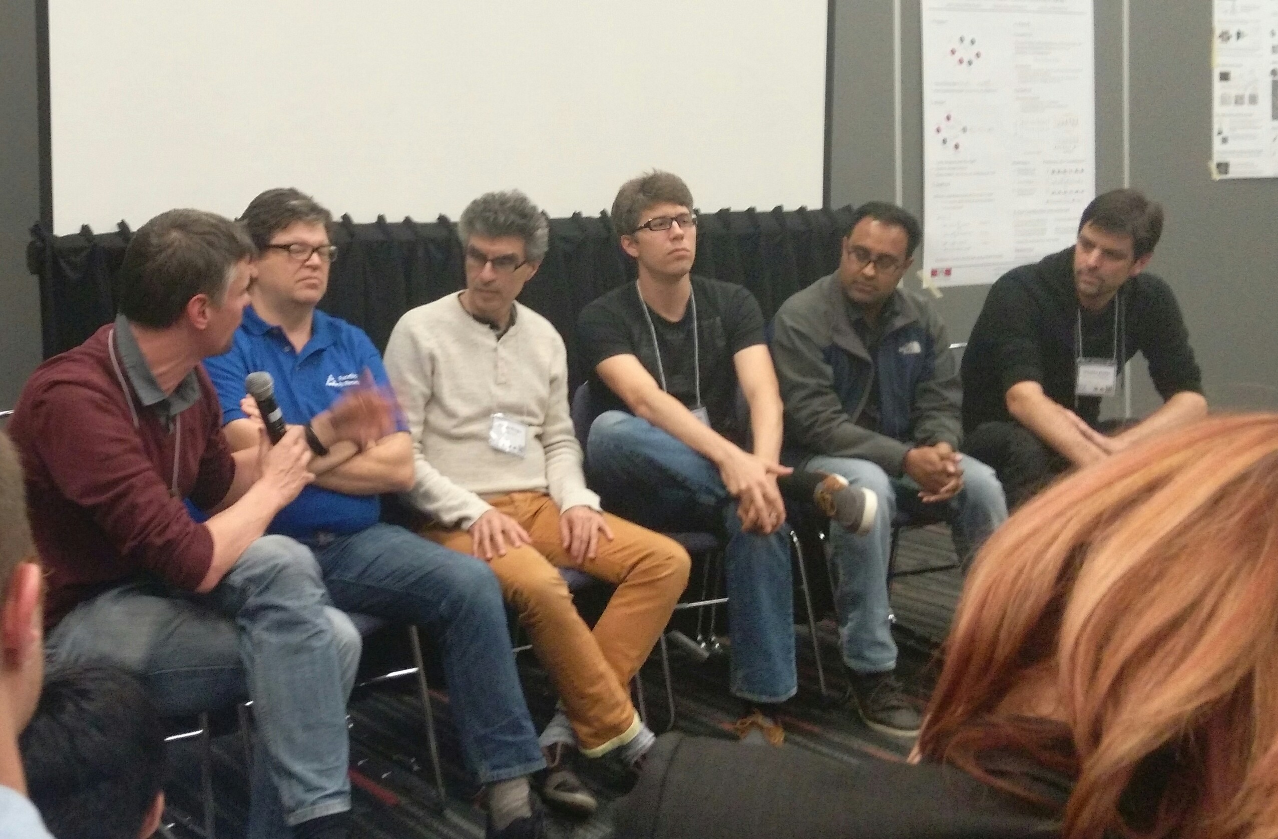
Figure: Panel session at the Statistical Methods for Understanding Neural Systems workshop.

It was a great workshop and with retrospect, I now think of it as the last event at NeurIPS that I attended that captured the spirit of those early meetings. It was in a small room, which was packed, and had a diversity of people from different fields, offering opinions in an open and constructive manner.

At the time the Human Brain project was recently launched, and I think it’s fair to say that most people in the room felt it was a colossal waste of money. The objective was to build a full simulation of the brain, and the counter point was, well even if you could do that, what do you learn by it.

Figure: Logo of the human brain project.

So by starting with the HBP logo, I was highlighting that even a “faithful” mechanistic model isn’t what we actually want, because it doesn’t enable us to understand the system. It’s just a mirror of the existing system.

Bernhard and I often talk about the issue of the kingdom that made maps that were more and more accurate. It features in a Jorge Luis Borges story, but predating that it appears in a Lewis Carroll story.

“What a useful thing a pocket-map is!” I remarked.

“That’s another thing we’ve learned from your Nation,” said Mein Herr, “map-making. But we’ve carried it much further than you. What do you consider the largest map that would be really useful?”

“About six inches to the mile.”

“Only six inches!” exclaimed Mein Herr. “We very soon got to six yards to the mile. Then we tried a hundred yards to the mile. And then came the grandest idea of all ! We actually made a map of the country, on the scale of a mile to the mile!”

“Have you used it much?” I enquired.

“It has never been spread out, yet,” said Mein Herr: “the farmers objected: they said it would cover the whole country, and shut out the sunlight ! So we now use the country itself, as its own map, and I assure you it does nearly as well.”

from Lewis Carroll, Sylvie and Bruno Concluded, Chapter XI, London, 1895

Figure: Rube Goldberg’s self operating napkin.

Also of interest to me was general properties of models, how we think about complex objects and I used a layered model of the computer network to represent the contextual idea of a model. That different layers are different ways of talking about the system (equivalent to different maps).

Figure: Network Layer models in Computer Science.

Figure: The mouse is a model, a physical model of how the world works. This drawing is a drawing of the mouse, so it’s a model of the model.

The point about these stories was to highlight something we talked about yesterday, that the model is contextual, like a good map. It needs to be something that we can use to answer a specific question. And like the different map scales are useful for walkers, cyclist and car drivers. And the different features on the map are also appropriate for different users, the right form of the model varies according to the user, or more broadly the context in which the user is operating.

I went on to argue that the rise of machine learning was being driven by the rise in data availability, as depicted in the graph below which shows digital data availability up to 2007. I suspect that to draw such a graph today would render the analogue component of data too small to fit.

Figure: The Global storage capacity between 1986 and 2007 Hilbert and López (2011)

Figure: Word cloud for big data.

One of the interesting features about machine learning is how it includes relatively simple (what I call weakly mechanistic) assumptions about the data. I think the interesting aspect of machine learning algorithms is the extent to w hich they allow the data to speak. For example the convolutional neural networks encode translation invariance.

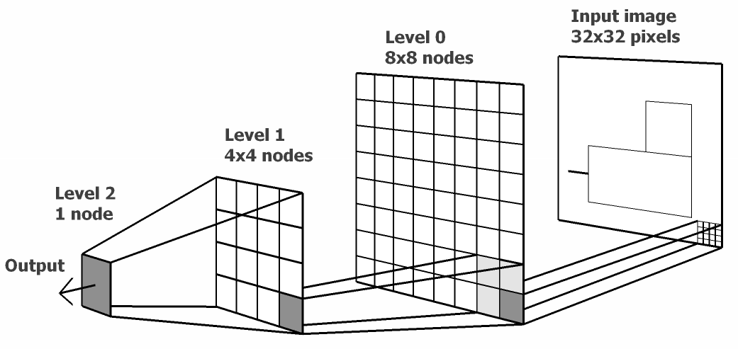
Figure: Hierarchical models for machine learning.

An additional model for intelligence comes from logic, which is often represented by Holmes and Watson, I could have been making one of two points here, and I don’t recall which it was. Either I was using the picture to remind me about graphical models, which are a very interesting way of introducing conditional independencies, or I was being rude about first order logic as a route to intelligence.

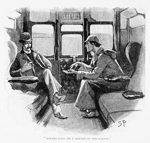
Figure: Holmes and Watson discussing a case.

One of the limitations of simplistic models of thought is nicely revealed by the “trolley problem” tropes, where human ethics is judged by asking for decisions around whether to take actions where a runaway trolley can either be diverted through some points, or by “throwing a fat man off a bridge”.

The Trolley Problem

[edit]

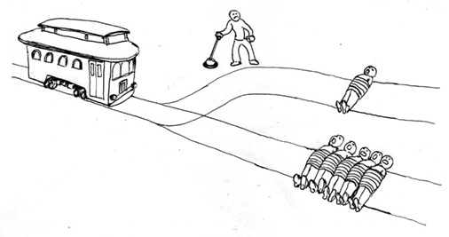
Figure: The trolley problem in its original form.

The Push and the Trolley

[edit]

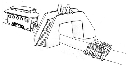
Figure: The trolley problem.

I later explored more ideas on these problems and the need for diversity in decision making blog post on in this blog post.

My memory is that I shifted to use the rest of the talk to reveal my secret interest in cognitive science, and was sharing some rough ideas from popular books and how these facets might map back to the way we perceive the world.

One of my major interests at the time (and in an ongoing way) was the manner in which the machines we were building were not sentient in the manner of the systems that we were being warned about by Elon Musk, Stephen Hawking, Nick Bostrom and others, they were non sentient. And therein lied the problem. I described these systems as “System Zero”, taking my cue from dual-process models in psychology which suggest that we have two thinking processes … fast and slow.

The Elephant and its Rider

[edit]

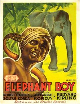
Figure: The elephant and its rider is an analogy used by Haidt to describe the difference between System One and System Two.

At the time one of my favourite approaches for thinking about these systems was from Jonathan Haidt’s book, where he suggests that the fast thinking side is an elephant, and the slow is a rider.

The Righteous Mind

[edit]

Figure: The Righteous Mind, by Jonathan Haidt, a social psychologist, uses the analogy of the elephant and the rider for dual process cognition.

Another book on these models is from the sports psychologist, Steve Peters, who was a former colleague from the University of Sheffield.

The Chimp Paradox

[edit]

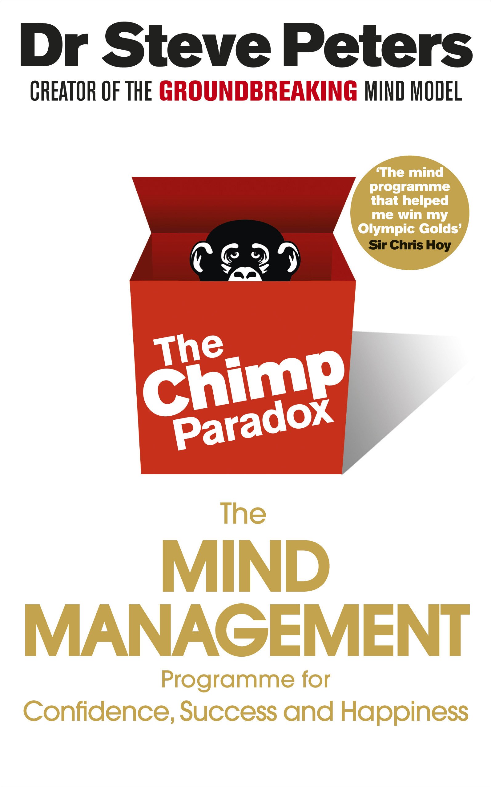
Figure: The Chimp Paradox is a variation of the dual process model used by the sports psychologist Steve Peters.

And I attended a talk of his where he suggested that these were just analogies that were highlighting work from early psychoanalysis such a Freud’s model of the Id, the Ego and the Superego, showing the long history of the dual process models (equivalent to the Chimp, the Human and the Computer in Peters’s model).

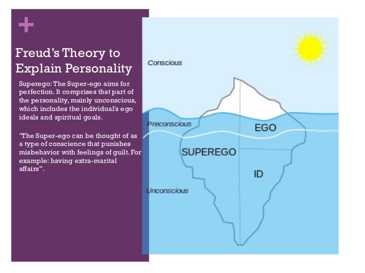
Figure: Freud’s model of the Id, the Ego and the Superego.

My suggestion was that the AI that we’d built was operating as a System Zero that was interfacing with our fast thinking, potentially to the detriment of our autonomy. There’s a blog post on blog post here where you can read more.

That process was being driven by the extent to which we were (and are) using data to create these “non-sentient” systems that were making decisions about us. From an ethical perspective this seemed problematic and our work on the data trusts initiative https://datatrusts.uk was inspired by these concerns. Currently we are supporting three pilot projects which attempt to give control of data back to the “citizens”. See also this Guardian article.

Other work I’m excited about that responds to these problems is Sylvie Delacroix’s book on habitual ethics. See also the youtube video below.

Figure: Launch event for Sylvie Delacroix’s book on habitual ethics which covers the challenges of ethical thinking when we are devolving decision making to habit.

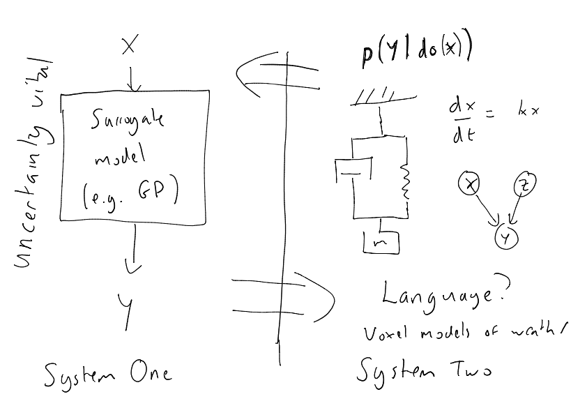
But at the conference, the main I deas I wanted to get across was how we might merge the data driven and the mechanistic approach by viewing System 2 as a mechanistic-like model, which is a new way of feeding data to the data-driven component.

This means that the relationship between System One and System Two would be like a surrogate model or an emulator, similar to work seen in Bayesian optimisation and other emulators. (Since then at Amazon the team, led by Andrei Paleyes and Javier Gonzalez built a framework for statistical emulation, Emukit, that we also place at the core of one of the Masters courses I teach on in Cambridge..

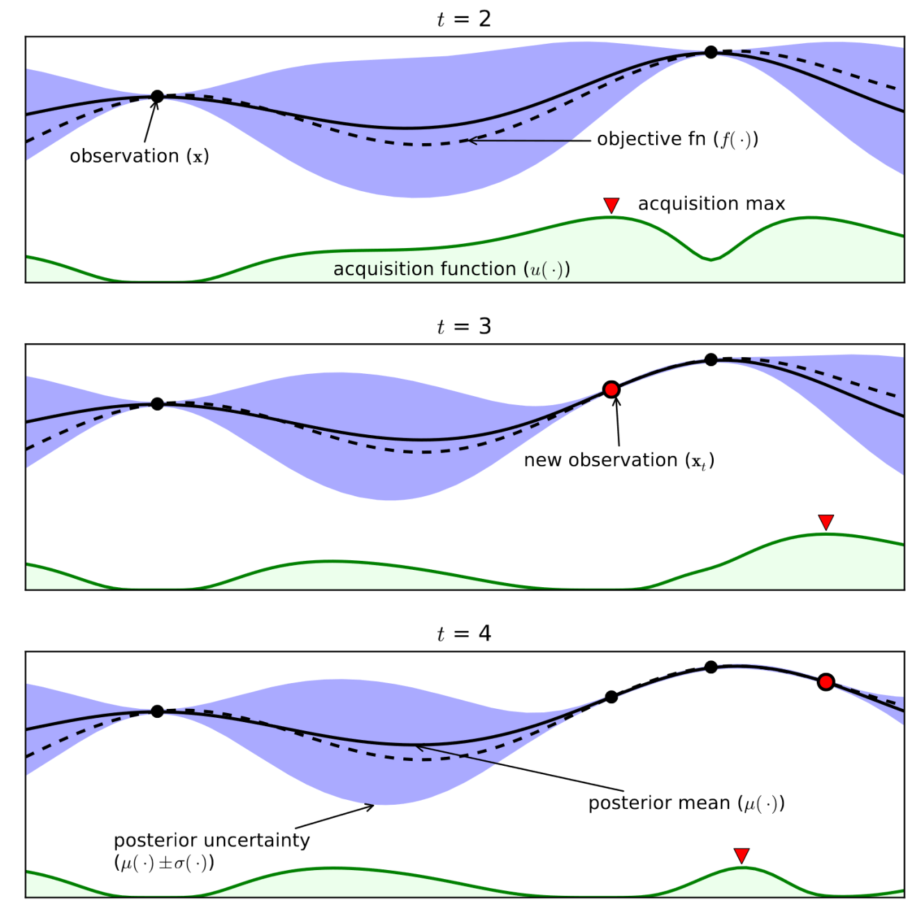
Figure: A representation of Bayesian optimisation, which is an approach where a surrogage model (or emulation) is used as a proxy to optimise rather than the slow to compute original system.

But key amoungst the surrogate, is the importance of “doubt”, the ability of System One to know when it doesn’t know, and take a sensible action. That was a theme I’d discussed in this blog post on blog post on Artificial Stupidity.

The final slide hints at the workshop we had yesterday, on Causal Digital Twins. Because what it says is that (roughly) our System Two could be thought of as a (causal) digital twin of the real world, that we use for planning. I think that relates very nicely to Bernhard’s Konrad Lorenz quote thinking is acting in an imagined space.

The theme for this section is caught by surprise, so what’s intesting to me is how much of what I was proposing in this talk is work that we continue to focus on today. However, if I was to be asked what caught me by surprise, it’s the extent to which the data driven approach can be extrapolated. I think the recent results aren’t a surprise given GPT-2, but I think if you’d asked any of the people on that panel at the time they wouldn’t have predicted the capabilities of GPT-2 with very little “weak mechanism” in the model.

Thanks!

For more information on these subjects and more you might want to check the following resources.

References

Hilbert, M., López, P., 2011. The world’s technological capcity to store, communicate and compute information. Science 332, 60–65. https://doi.org/10.1126/science.1200970