Abstract

In this talk I will introduce the importance of uncertainty in decision making and describe how it provides a mathematical justification for procrastination through the game of Kappenball.

Laplace’s Demon

Figure: English translation of Laplace’s demon, taken from the Philosophical Essay on probabilities Laplace (1814) pg 3.

One way of viewing what Laplace is saying is that we can take “the forces by which nature is animated” or our best mathematical/computational abstraction of that which we would call the model and combine it with the “respective situation of the beings who compose it” which I would refer to as the data and if we have an “intelligence sufficiently vast enough to submit these data to analysis,” or sufficient compute then we would have a system for which “nothing would be uncertain and the future, as the past, would be present in its eyes,” or in other words we can make a prediction. Or more succinctly put we have

Laplace’s demon has been a recurring theme in science, we can also find it in Stephen Hawking’s book A Brief History of Time (A brief history of time, 1988).

If we do discover a theory of everything … it would be the ultimate triumph of human reason-for then we would truly know the mind of God

Stephen Hawking in A Brief History of Time 1988

But is it really that simple? Do we just need more and more accurate models and more and more data?

Emergent Behaviour

Cellular Automata

Cellular automata are systems of cells that evolve according to fixed rules. The rules depend on the current state of cells and their neighbors. We’ll explore both one-dimensional (Wolfram) and two-dimensional (Conway) cellular automata. First, we’ll set up some base functionality that both types share.

These base classes and functions provide:

1. A flexible grid structure that works for both 1D and 2D automata
2. Consistent array access patterns
3. Grid visualization tools
4. Support for highlighting interesting cells or patterns

We’ll build on this foundation to implement both Wolfram’s elementary one dimensional cellular automata and later Conway’s two dimensional Game of Life.

These diagram generation functions maintain consistent styling while providing specialized visualizations for:

1. Wolfram rule definitions and their outcomes
2. Game of Life rules and their effects

They work with the base Grid class but provide custom layouts specific to teaching and explaining the rules of each system.

Life Rules

John Conway’s game of life is a cellular automaton where the cells obey three very simple rules. The cells live on a rectangular grid, so that each cell has 8 possible neighbors.

loneliness

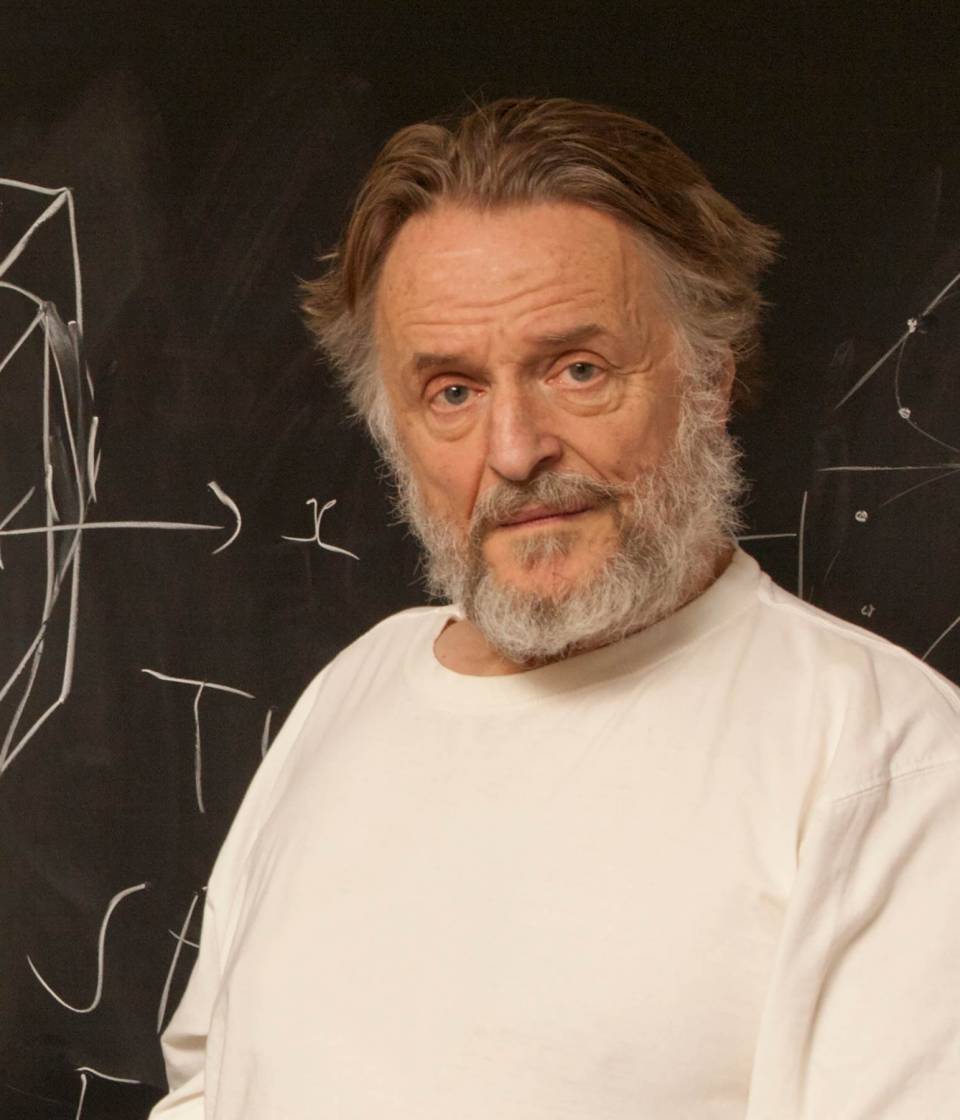
Figure: ‘Death’ through loneliness in Conway’s game of life. If a cell is surrounded by less than three cells, it ‘dies’ through loneliness.

The game proceeds in turns, and at each location in the grid is either alive or dead. Each turn, a cell counts its neighbors. If there are two or fewer neighbors, the cell ‘dies’ of ‘loneliness.’

overcrowding

Figure: ‘Death’ through overpopulation in Conway’s game of life. If a cell is surrounded by more than three cells, it ‘dies’ through loneliness.

If there are four or more neighbors, the cell ‘dies’ from ‘overcrowding.’ If there are three neighbors, the cell persists, or if it is currently dead, a new cell is born.

birth

Figure: Birth in Conway’s life. Any position surrounded by precisely three live cells will give birth to a new cell at the next turn.

And that’s it. Those are the simple ‘physical laws’ for Conway’s game.

Game of Life Implementation

Now that we understand the rules of Life, let’s implement them. Each cell’s fate is determined by counting its eight neighbors and applying Conway’s rules.

The implementation above provides: 1. Neighbor counting with different boundary conditions 2. Rule application following Conway’s specifications 3. Support for both periodic and fixed boundaries 4. History tracking for visualization 5. Flexible initial state configuration

This base implementation will be essential when we combine it with Wolfram automata, as we’ll need to modify the boundary conditions to interact with the Wolfram rules.

Figure: Evolution of a simple oscillator (blinker) in the Game of Life.

This implementation will serve as the foundation for our exploration of Life patterns and ultimately for our hybrid system combining Life with Wolfram automata. The key is the flexibility in boundary conditions, which will allow us to interface with Wolfram rules at the edges.

Spaceships, oscillators and static patterns

The game leads to patterns emerging, some of these patterns are static, but some oscillate in place, with varying periods. Others oscillate, but when they complete their cycle they’ve translated to a new location, in other words they move. In Life the former are known as oscillators and the latter as spaceships.

Pattern Analysis

Before looking at specific examples, let’s understand how these patterns behave. Life patterns can be classified by their periodic behavior and movement: - Static patterns remain unchanged from one generation to the next - Oscillators return to their initial state after a fixed number of generations (their period) - Spaceships combine oscillation with translation, moving across the grid while cycling through their states

Each pattern can be characterized by: - Its period (how many steps before it repeats) - Its translation (how far it moves each period) - Its velocity (translation per period)

import matplotlib.pyplot as plt
from matplotlib.animation import FuncAnimation

John Horton Conway, as the creator of the game of life, could be seen somehow as the god of this small universe. He created the rules. The rules are so simple that in many senses he, and we, are all-knowing in this space. But despite our knowledge, this world can still ‘surprise’ us. From the simple rules, emergent patterns of behaviour arise.

Glider (1969)

Figure: Left A Glider pattern discovered 1969 by Richard K. Guy. Right. John Horton Conway, creator of Life (1937-2020). The glider is an oscillator that moves diagonally after creation.

The glider was ‘discovered’ in 1969 by Richard K. Guy. What do we mean by discovered in this context? Well, as soon as the game of life is defined, objects such as the glider do somehow exist, but the many configurations of the game mean that it takes some time for us to see one and know it exists. This means, that despite being the creator, Conway, and despite the rules of the game being simple, and despite the rules being deterministic, we are not ‘omniscient’ in any simplistic sense. It requires computation to ‘discover’ what can exist in this universe once it’s been defined.

Figure: The Gosper glider gun is a configuration that creates gliders. A new glider is released after every 30 turns.

These patterns had to be discovered, in the same way that a scientist might discover a disease, or an explorer a new land. For example, the Gosper glider gun was discovered by Bill Gosper in 1970. It is a pattern that creates a new glider every 30 turns of the game.

Loafer (2013)

Figure: Left A Loafer pattern discovered by Josh Ball in 2013. Right. John Horton Conway, creator of Life (1937-2020).

Despite widespread interest in Life, some of its patterns were only very recently discovered like the Loafer, discovered in 2013 by Josh Ball. So, despite the game having existed for over forty years, and the rules of the game being simple, there are emergent behaviors that are unknown.

Laplace’s Gremlin

The curve described by a simple molecule of air or vapor is regulated in a manner just as certain as the planetary orbits; the only difference between them is that which comes from our ignorance. Probability is relative, in part to this ignorance, in part to our knowledge. We know that of three or greater number of events a single one ought to occur; but nothing induces us to believe that one of them will occur rather than the others. In this state of indecision it is impossible for us to announce their occurrence with certainty. It is, however, probable that one of these events, chosen at will, will not occur because we see several cases equally possible which exclude its occurrence, while only a single one favors it.

— Pierre-Simon Laplace (Laplace, 1814), pg 5

The representation of ignorance through probability is the true message of Laplace, I refer to this message as “Laplace’s gremlin,” because it is the gremlin of uncertainty that interferes with the demon of determinism to mean that our predictions are not deterministic.

Our separation of the uncertainty into the data, the model and the computation give us three domains in which our doubts can creep into our ability to predict. Over the last three lectures we’ve introduced some of the basic tools we can use to unpick this uncertainty. You’ve been introduced to, (or have yow reviewed) Bayes’ rule. The rule, which is a simple consequence of the product rule of probability, is the foundation of how we update our beliefs in the presence of new information.

The real point of Laplace’s essay was that we don’t have access to all the data, we don’t have access to a complete physical understanding, and as the example of the Game of Life shows, even if we did have access to both (as we do for “Conway’s universe”) we still don’t have access to all the compute that we need to make deterministic predictions. There is uncertainty in the system which means we can’t make precise predictions.

Gremlins are imaginary creatures used as an explanation of failure in aircraft, causing crashes. In that sense the Gremlin represents the uncertainty that a pilot felt about what might go wrong in a plane which might be “theoretically sound” but in practice is poorly maintained or exposed to conditions that take it beyond its design criteria. Laplace’s gremlin is all the things that your model, data and ability to compute don’t account for bringing about failures in your ability to predict. Laplace’s gremlin is the uncertainty in the system.

Figure: Gremlins are seen as the cause of a number of challenges in this World War II poster.

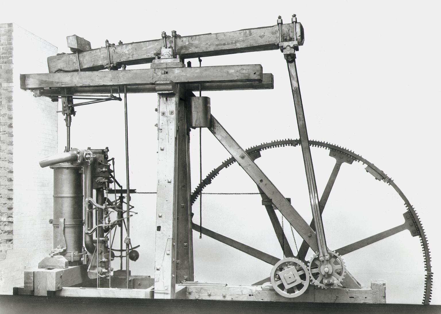
Boulton and Watt’s Lap Engine

Lap Engine (1788)

total energy
=
available energy
+
temperature
\(\times\)
entropy

Figure: James Watt’s Lap Engine which incorporates many of his innovations to the steam engine, making it more efficient.

Brownian Motion and Wiener

Robert Brown was a botanist who was studying plant pollen in 1827 when he noticed a trembling motion of very small particles contained within cavities within the pollen. He worked hard to eliminate the potential source of the movement by exploring other materials where he found it to be continuously present. Thus, the movement was not associated, as he originally thought, with life.

In 1905 Albert Einstein produced the first mathematical explanation of the phenomenon. This can be seen as our first model of a ‘curve of a simple molecule of air.’ To model the phenomenon Einstein introduced stochasticity to a differential equation. The particles were being peppered with high-speed water molecules, that was triggering the motion. Einstein modelled this as a stochastic process.

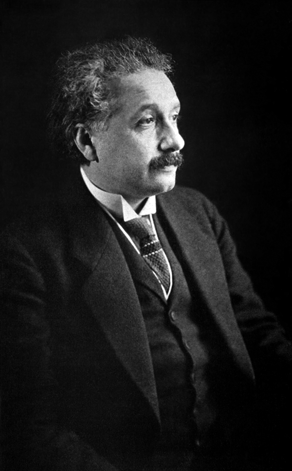
Figure: Albert Einstein’s 1905 paper on Brownian motion introduced stochastic differential equations which can be used to model the ‘curve of a simple molecule of air.’

Norbert Wiener was a child prodigy, whose father had schooled him in philosophy. He was keen to have his son work with the leading philosophers of the age, so at the age of 18 Wiener arrived in Cambridge (already with a PhD). He was despatched to study with Bertrand Russell but Wiener and Russell didn’t get along. Wiener wasn’t persuaded by Russell’s ideas for theories of knowledge through logic. He was more aligned with Laplace and his desire for a theory of ignorance. In is autobiography he relates it as the first thing he could see his father was proud of (at around the age of 10 or 11) (Wiener, 1953).

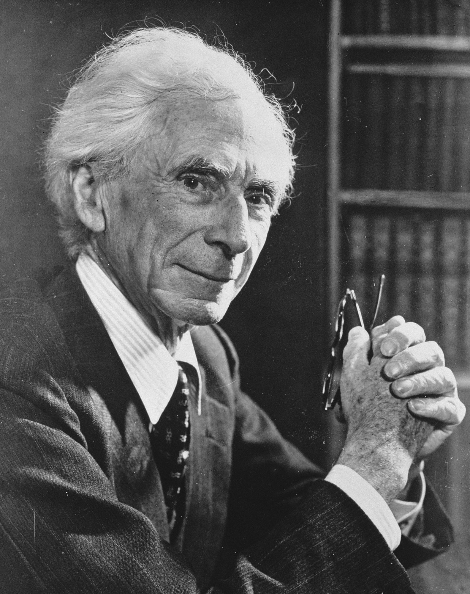
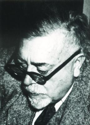
Figure: Bertrand Russell (1872-1970), Albert Einstein (1879-1955), Norbert Wiener, (1894-1964)

But Russell (despite also not getting along well with Wiener) introduced Wiener to Einstein’s works, and Wiener also met G. H. Hardy. He left Cambridge for Göttingen where he studied with Hilbert. He developed the underlying mathematics for proving the existence of the solutions to Einstein’s equation, which are now known as Wiener processes.

Figure: Brownian motion of a large particle in a group of smaller particles. The movement is known as a Wiener process after Norbert Wiener.

Figure: Norbert Wiener (1894 - 1964). Founder of cybernetics and the information era. He used Gibbs’s ideas to develop a “theory of ignorance” that he deployed in early communication. On the right is Wiener’s wartime report that used stochastic processes in forecasting with applications in radar control (image from Coales and Kane (2014)).

Wiener himself used the processes in his work. He was focused on mathematical theories of communication. Between the world wars he was based at Massachusetts Institute of Technology where the burgeoning theory of electrical engineering was emerging, with a particular focus on communication lines. Winer developed theories of communication that used Gibbs’s entropy to encode information. He also used the ideas behind the Wiener process for developing tracking methods for radar systems in the second world war. These processes are what we know of now as Gaussian processes (Wiener (1949)).

James Clerk Maxwell

Ludwig Boltzmann

Josiah Willard Gibbs

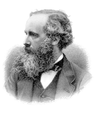
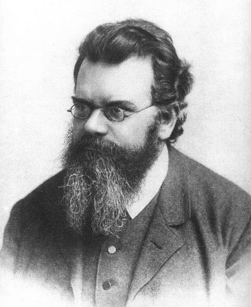
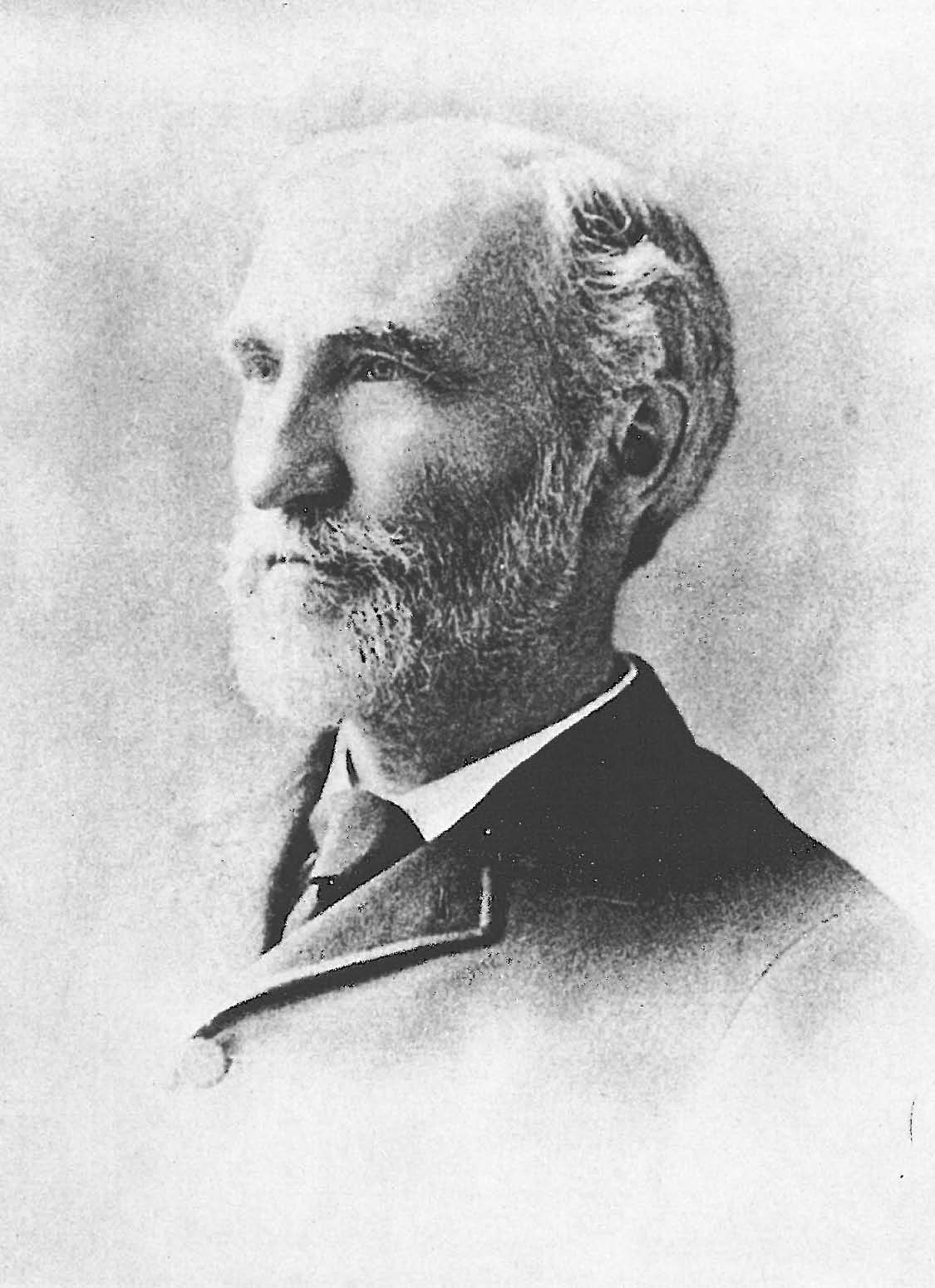
Figure: James Clerk Maxwell (1831-1879), Ludwig Boltzmann (1844-1906) Josiah Willard Gibbs (1839-1903)

Entropy Billiards

Velocity-bin entropy:

New Ball Pause Skip 1000s Histogram

Figure: Bernoulli’s simple kinetic models of gases assume that the molecules of air operate like billiard balls. The displayed entropy is the Shannon entropy of the observed velocity histogram (a coarse-grained proxy, not full thermodynamic entropy).

Maxwell’s Demon

Figure: Maxwell’s demon opens and closes a door which allows fast particles to pass from left to right and slow particles to pass from right to left. This makes the left hand side colder than the right.

Velocity-bin entropy:

New Ball Pause Skip 1000s Histogram

Figure: Maxwell’s Demon. The demon decides balls are either cold (blue) or hot (red) according to their velocity. Balls are allowed to pass the green membrane from right to left only if they are cold, and from left to right only if they are hot. The displayed entropy is the Shannon entropy of the velocity histogram (a coarse-grained proxy, not full thermodynamic entropy).

Procrastination

Kappenball

Score:

Energy:

New Ball Pause

Figure: Kappen Ball

If you want to complete a task, should you do it now or should you put it off until tomorrow? Despite being told to not delay tasks, many of us are deadline driven. Why is this?

Kappenball is a simple game that illustrates that this behaviour can be optimal. It is inspired by an example in stochastic optimal control by Bert Kappen. The game is as follows: you need to place a falling balloon into one of two holes, but if the balloon misses the holes it will pop on pins placed in the ground. In ‘deterministic mode,’ the balloon falls straight towards the ground and the game is easy. You simply choose which hole to place the ball in, and you can start to place it there as soon as the ball appears at the top of the screen. The game becomes more interesting as you increase the uncertainty. In Kappenball, the uncertainty takes the form of the balloon being blown left and right as it falls. This movement means that it is not sensible to decide early on which hole to place the balloon in. A better strategy is to wait and see which hole the ball falls towards. You can then place it in that hole using less energy than in deterministic mode. Sometimes, the ball even falls into the hole on its own, and you don’t have to expend any energy, but it requires some skill to judge when you need to intervene. For this system Bert Kappen has shown mathematically that the best solution is to wait until the ball is close to the hole before you push it in. In other words, you should be deadline driven.

In fact, it seems here uncertainty is a good thing, because on average you’ll get the ball into the hole with less energy (by playing intelligently, and being deadline driven!) than you do with `deterministic mode’. It requires some skill to do this, more than the deterministic system, but by using your resources intelligently you can get more out of the system. However, if the uncertainty increases too much then regardless of your skill, you can’t control the ball at all.

This simple game explains many of the behaviours we exhibit in real life. If a system is completely deterministic, then we can make a decision early on and be sure that the ball will ‘drop in the hole.’ However, if there is uncertainty in a system, it can make sense to delay our decision making until we’ve seen how events ‘pan out.’ Be careful though, as we also see that when the uncertainty is large, if you don’t have the resources or the skill to be deadline-driven the uncertainty can overwhelm you and events can quickly move beyond our control.

Information and Embodiment

Claude Shannon

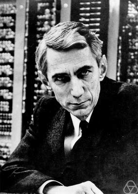
Figure: Claude Shannon (1916-2001)

bits/min	billions	2,000
billion calculations/s	~100	a billion
embodiment	20 minutes	5 billion years

Figure: Embodiment factors are the ratio between our ability to compute and our ability to communicate. Relative to the machine we are also locked in. In the table we represent embodiment as the length of time it would take to communicate one second’s worth of computation. For computers it is a matter of minutes, but for a human, it is a matter of thousands of millions of years.

Figure: Conversation relies on internal models of other individuals.

Figure: Misunderstanding of context and who we are talking to leads to arguments.

Embodiment factors imply that, in our communication between humans, what is not said is, perhaps, more important than what is said. To communicate with each other we need to have a model of who each of us are.

To aid this, in society, we are required to perform roles. Whether as a parent, a teacher, an employee or a boss. Each of these roles requires that we conform to certain standards of behaviour to facilitate communication between ourselves.

Control of self is vitally important to these communications.

The consequences between this mismatch of power and delivery are to be seen all around us. Because, just as driving an F1 car with bicycle wheels would be a fine art, so is the process of communication between humans.

If I have a thought and I wish to communicate it, I first need to have a model of what you think. I should think before I speak. When I speak, you may react. You have a model of who I am and what I was trying to say, and why I chose to say what I said. Now we begin this dance, where we are each trying to better understand each other and what we are saying. When it works, it is beautiful, but when mis-deployed, just like a badly driven F1 car, there is a horrible crash, an argument.

Stories, between humans.

I have a great dislike for Russell; I cannot explain it completely, but I feel a detestation for the man. As far as any sympathy with me, or with anyone else, I believe, he is an iceberg. His mind impresses one as a keen, cold, narrow logical machine, that cuts the universe into neat little packets, that measure, as it were, just three inches each way. His type of mathematical analysis he applies as a sort of Procrustean bed to the facts, and those that contain more than his system provides for, he lops short, and those that contain less, he draws out.

Norbert Wiener in a letter to his family, 1913

Heider and Simmel (1944)

Figure: Fritz Heider and Marianne Simmel’s video of shapes from Heider and Simmel (1944).

Fritz Heider and Marianne Simmel’s experiments with animated shapes from 1944 (Heider and Simmel, 1944). Our interpretation of these objects as showing motives and even emotion is a combination of our desire for narrative, a need for understanding of each other, and our ability to empathize. At one level, these are crudely drawn objects, but in another way, the animator has communicated a story through simple facets such as their relative motions, their sizes and their actions. We apply our psychological representations to these faceless shapes to interpret their actions (Heider, 1958).

See also a recent review paper on Human Cooperation by Henrich and Muthukrishna (2021). See Lawrence (2024) psychological representation p. 326–329, 344–345, 353, 361, 367.

Computer Conversations

Figure: Conversation relies on internal models of other individuals.

Figure: Misunderstanding of context and who we are talking to leads to arguments.

Similarly, we find it difficult to comprehend how computers are making decisions. Because they do so with more data than we can possibly imagine.

In many respects, this is not a problem, it’s a good thing. Computers and us are good at different things. But when we interact with a computer, when it acts in a different way to us, we need to remember why.

Just as the first step to getting along with other humans is understanding other humans, so it needs to be with getting along with our computers.

Embodiment factors explain why, at the same time, computers are so impressive in simulating our weather, but so poor at predicting our moods. Our complexity is greater than that of our weather, and each of us is tuned to read and respond to one another.

Their intelligence is different. It is based on very large quantities of data that we cannot absorb. Our computers don’t have a complex internal model of who we are. They don’t understand the human condition. They are not tuned to respond to us as we are to each other.

Embodiment factors encapsulate a profound thing about the nature of humans. Our locked in intelligence means that we are striving to communicate, so we put a lot of thought into what we’re communicating with. And if we’re communicating with something complex, we naturally anthropomorphize them.

We give our dogs, our cats, and our cars human motivations. We do the same with our computers. We anthropomorphize them. We assume that they have the same objectives as us and the same constraints. They don’t.

This means, that when we worry about artificial intelligence, we worry about the wrong things. We fear computers that behave like more powerful versions of ourselves that will struggle to outcompete us.

In reality, the challenge is that our computers cannot be human enough. They cannot understand us with the depth we understand one another. They drop below our cognitive radar and operate outside our mental models.

The real danger is that computers don’t anthropomorphize. They’ll make decisions in isolation from us without our supervision because they can’t communicate truly and deeply with us.

See Lawrence (2024) telepathy p. 248-50. See Lawrence (2024) anthropomorphization (‘anthrox’) p. 30-31, 90-91, 93-4, 100, 132, 148, 153, 163, 216-17, 239, 276, 326, 342.

Networked Interactions

Our modern society intertwines the machine with human interactions. The key question is who has control over these interfaces between humans and machines.

Figure: Humans and computers interacting should be a major focus of our research and engineering efforts.

So the real challenge that we face for society is understanding which systemic interventions will encourage the right interactions between the humans and the machine at all of these interfaces.

Figure: Humans use culture, facts and ‘artefacts’ to communicate.

Richard Feynmann on Doubt

One thing is I can live with is doubt, and uncertainty and not knowing. I think it’s much more interesting to live with not knowing than to have an answer that might be wrong.

Richard P. Feynmann in the The Pleasure of Finding Things Out 1981.

Thanks!

For more information on these subjects and more you might want to check the following resources.

• company: Trent AI
• book: The Atomic Human
• twitter: @lawrennd
• podcast: The Talking Machines
• newspaper: Guardian Profile Page
• blog: http://inverseprobability.com

References