In this post we’ll provide a general introduction to machine learning, which tries to highlight the underlying technical challenges and where we have solutions. Machine learning is the principle technology underpinning the recent advances in artificial intelligence. But what is machine learning? And why is it important?

Machine learning is perhaps the principal technology behind two emerging domains: data science and artificial intelligence. The rise of machine learning is coming about through the availability of data and computation, but machine learning methdologies are fundamentally dependent on models.

\[\text{data} + \text{model} \xrightarrow{\text{compute}} \text{prediction}\]

The emergence of machine learning is closely tied to the emergence of widely available data.

Large amounts of data and high interconnection bandwidth mean that we receive much of our information about the world around us through computers.

Economists try to measure productivity, one of the ways we can become more productive is by becoming more efficient. For example, moving from gathering food to settled agriculture. In the modern era one approach to becoming more efficient is automation of processes like manufacturing production lines. The manufacturing process is decomposed into a series of mechanical or manual processes each of which is applied sequentially.

Manufacturing processes consist of production lines and robotic automation. Logistics can also be decomposed into the supply chain processes. Whether it’s manufacturing or logistics, efficiency can be improved by automating components of the processes to improve the flow of goods.

An interesting challenge for modern society is the management of both the flow of goods and the flow of information. The flow of information is also highly automated. Processing of data is decomposed into stages in computer code.

In these processing pipelines, manufacturing, logistics or data management, the overall pipeline normally also requires human intervention from an operator. These interventions can create bottlenecks and slow the process of automation. Machine learning is the key technology in automating these manual stages.

The human interventions that were easy to replicate with technology have already been replaced. The components that still require human intervention are the knottier problems. Often they represent components that are difficult, or impossible, to decompose into stages which could then be further automated. In that sense these components are process-atoms. In manufacturing or logistics settings these atoms involve the sort of flexible manual skills that we cannot replicate with current robotic technology. They require emulation of a human’s motor skills. In information processing settings these atoms require emulation of our cognitive skills. For example, our ability to mentally process an image or some text.

Machine learning is a field dedicated to replicating such processes through the direct use of data. It is an approach to splitting these process-atoms so that they too be automated. In machine learning we aim to emulate cognitive processes through the use of data. Machine learning also uses data to provide new approaches in control and optimization that should allow for emulation of human motor skills.

A key idea in machine learning is to emulate the process as a mathematical function. Each function has a set of parameters which control its behavior. Learning is the process of changing these parameters to change the shape of the function to make it more representative of the data. Our choice of which class of mathematical functions we use is a vital component of our model.

Example of prediction: The Olympic gold medalist in the marathon’s pace is predicted using a regression fit. In this case the mathematical function is directly predicting the pace of the winner as a function of the year of the Olympics.

Machine learning has risen to prominence as the principal technology underlying the recent advances in artificial intelligence techniques. It takes a different approach to that developed in classical artificial intelligence (sometimes referred to as “good old fashioned AI” or GOFAI). GOFAI relied on symbolic logic as its mathematical engine. Early AI used expert systems: a set of logical rules implemented to reconstruct expertise. For example, rules to decide whether or not someone has cancer. Such rules prove hard to specify for very complex processes.¹

Data Science

We can split applications of machine learning broadly into data science and artificial intelligence. We define the field of data science to be the challenge of making sense of the large volumes of data that have now become available through the increase in sensors and the large interconnection of the internet. Phenomena variously known as “big data” or “the internet of things”. Data science differs from traditional statistics in that this data is not necessarily collected with a purpose or experiment in mind. It is collected by happenstance, and we try and extract value from it later. In classical statistics the question is formed first, and data is collected to answer the question. Karl Popper, the philosopher of science, once put the challenge of model (or question) and experiment (or data) as being similar to the challenge of the chicken and the egg. Which comes first? His answer is that they co-evolve. And a similar answer should apply to the model and the data. But in classical statistics it was normally the question (which could be encoded in a model) that comes first. In modern data science it is often the data that comes first. Regardless, to truly answer questions to our satisfaction several stages of modelling and data collection are likely to be required. This naturally implies that classical statistical analyses are as important as ever in this domain.

Artificial Intelligence

Artificial intelligence on the other hand is a field with its origins in Cybernetics. The challenge in artificial intelligence is to recreate “intelligent” behaviour. In particular there is a focus on having machines emulate the capabilities of humans. Machine learning has become important in this domain because of the success of data-driven artificial intelligence. In data-driven artificial intelligence, rather than solving a challenge in intelligence from first principles, we simply acquire data that guides us to the solution of the problem. Often such data is acquired from humans, and the computer is given the task of reconstructing that data. This is where machine learning techniques come in. Machine learning focuses on emulating the data creation process by combining a model with the data. The model incorporates assumptions about the data generating process. But unlike physical models (e.g. differential equation models) the assumptions are typically only weak. Smoothness assumptions are common, and the success of convolutional neural networks is driven by the assumptions they can encode about how an image is structured.

Machine Learning

Machine learning takes the different approach of observing a system in practice and emulating its behavior with mathematics. One of the design aspects in designing machine learning solutions is where to put the mathematical function. Obtaining complex behavior in the resulting system can require some imagination in the design process. We will give an overview of the approaches that people take using the classical three subdivisions of the field: supervised learning, unsupervised learning and reinforcement learning. Each of these approaches uses the mathematical functions in a different way. Below we will introduce each of these learning challenges and explore how the mathematical function is deployed.

Supervised Learning

Supervised learning is one of the most widely deployed machine learning technologies, and a particular domain of success has been classification. Classification is the process of taking an input (which might be an image) and categorizing it into one of a number of different classes (e.g. dog or cat). This simple idea underpins a lot of machine learning. By scanning across the image we can also determine where the animal is in the image.

Classification is perhaps the technique most closely assocated with machine learning. In the speech based agents, on-device classifiers are used to determine when the wake word is used. A wake word is a word that wakes up the device. For the Amazon Echo it is “Alexa”, for Siri it is “Hey Siri”. Once the wake word detected with a classifier, the speech can be uploaded to the cloud for full processing, the speech recognition stages.

A major breakthrough in image classification came in 2012 with the ImageNet result of Alex Krizhevsky, Ilya Sutskever and Geoff Hinton from the University of Toronto. ImageNet is a large data base of 14 million images with many thousands of classes. The data is used in a community-wide challenge for object categorization. Krizhevsky et al used convolutional neural networks to outperform all previous approaches on the challenge. They formed a company which was purchased shortly after by Google. This challenge, known as object categorisation, was a major obstacle for practical computer vision systems. Modern object categorization systems are close to human performance.

In supervised learning the inputs, $\mathbf{x}$, are mapped to a label, $y$, through a function $f(\cdot)$ that is dependent on a set of parameters, $\mathbf{w}$,

\[y = f(\mathbf{x}; \mathbf{w}).\]

The function $f(\cdot)$ is known as the prediction function. The key challenges are (1) choosing which features, $\mathbf{x}$, are relevant in the prediction, (2) defining the appropriate class of function, $f(\cdot)$, to use and (3) selecting the right parameters, $\mathbf{w}$.

Feature Selection

Feature selection is a critical stage in the algorithm design process. In the Olympic prediction example above we’re only using time to predict the the pace of the runners. In practice we might also want to use characteristics of the course: how hilly it is, what the temperature was when the race was run. In 1904 the runners actually got lost during the race. Should we include ‘lost’ as a feature? It would certainly help explain the particularly slow time in 1904. The features we select should be ones we expect to correlate with the prediction. In statistics, these features are even called predictors which highlights their role in developing the prediction function. For Facebook newsfeed, we might use features that include how close your friendship is with the poster, or how often you react to that poster, or whether a photo is included in the post.

Sometimes we use feature selection algorithms, algorithms that automate the process of finding the features that we need. Classification is often used to rank search results, to decide which adverts to serve or, at Facebook, to determine what appears at the top of your newsfeed. In the Facebook example features might include how many likes a post has had, whether it has an image in it, whether you regularly interact with the friend who has posted. A good newsfeed ranking algorithm is critical to Facebook’s success, just as good ad serving choice is critical to Google’s success. These algorithms are in turn highly dependent on the feature sets used. Facebook in particular has made heavy investments in machine learning pipelines for evaluation of the feature utility.

Class of Function, $f(\cdot)$

By class of function we mean, what are the characteristics of the mapping between $\mathbf{x}$ and $y$. Often we might choose it to be a smooth function. Sometimes we will choose it to be a linear function. If the prediction is a forecast, for example the demand of a particular product, then the function would need some periodic components to reflect seasonal or weekly effects.

In the ImageNet challenge the input, $\mathbf{x}$, was in the form of an image. And the form of the prediction function was a convolutional neural network (more on this later). A convolutional neural network introduces invariances into the function that are particular to image classification. An invariance is a transformation of the input that we don’t want to effect the output. For example, a cat in an image is still a cat no matter where it’s located in the image (translation). The cat is also a cat regardless of how large it is (scale), or whether it’s upside-down (rotation). Convolutional neural networks encode these invariances: scale invariance, rotation invariance and translation invariance; in the mathematical function.

Encoding invariance in the prediction function is like encoding knowledge in the model. If we don’t specify these invariances then the model must learn them. This will require a lot more data to achieve the same performance, making the model less data efficient. Note that one invariance that is not encoded in a convolutional network is invariance to camera type. As a result practitioners need to be careful to ensure that their training data is representative of the type of cameras that will be used when the model is deployed.

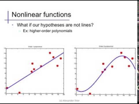
In general the prediction function could be any set of parameterized functions. In the Olympic marathon data example above we used a polynomial fit,

\[f(x) = w_0 + w_1 x+ w_2 x^2 + w_3 x^3 + w_4 x^4.\]

The Olympic example is also a supervised learning challenge. But it is a regression problem. A regression problem is one where the output is a continuous value (such as the pace in the marathon). In classification the output is constrained to be discrete. For example classifying whether or not an image contains a dog implies the output is binary. An early example of a regression problem used in machine learning was the Tecator data, where the fat, water and protein content of meat samples was predicted as a function of the absorption of infrared light.

Parameter Estimation

Once we have a set of features and the class of functions we use is determined we need to find the parameters of the model.

The parameters of the model, $\mathbf{w}$, are estimated by specifying an objective function. The objective function specifies the quality of the match between the prediction function and the training data. In supervised learning the objective function incorporates both the input data (in the ImageNet data the image, in the Olympic marathon data the year of the marathon) and a label.

The label is where the term supervised learning comes from. The idea being that a supervisor, or annotator, has already looked at the data and given it labels. For regression problem, a typical objective function is the squared error,

\[E(\mathbf{w}) = \sum_{i=1}^n (y_i - f(\mathbf{x}_i))^2\]

where the data is provided to us as a set of $n$ inputs, $\mathbf{x}_1$, $\mathbf{x}_2$, $\mathbf{x}_3$, $\dots$, $\mathbf{x}_n$ each one with an associated label, $y_1$, $y_2$, $y_3$, $\dots$, $y_n$. Sometimes the label is cheap to acquire. For example in Newsfeed ranking Facebook are acquiring a label each time a user clicks on a post in their Newsfeed. Similarly in ad-click prediction labels are obtained whenever an advert is clicked. More generally though, we have to employ human annotators to label the data. For example, ImageNet, the breakthrough deep learning result was annotated using Amazon’s Mechanical Turk. Without such large scale human input we would not have the breakthrough results on image categorization we have today.

Some tasks are easier to annotate than others. For example, in the Tecator data, to acquire the actual values of water, protein and fat content in the meat samples further experiments may be required. It is not simply a matter of human labelling. Even if the task is easy for humans to solve there can be problems. For example, humans will extrapolate the context of an image. A colleague mentioned once to me a challenge where humans were labelling images as containing swimming pools, even though none was visible, because they could infer there must be a pool nearby, perhaps because there are kids wearing bathing suits. But there is no swimming pool in the image for the computer to find. The quality of any machine learning solution is very sensitive to the quality of annotated data we have. Investing in processes and tools to improve annotation of data is therefore priority for improving the quality of machine learning solutions.

There can also be significant problems with misrepresentation in the data set. If data isn’t collected carefully, then it can reflect biases about the population that we don’t want our models to have. For example, if we design a face detector using Californians may not perform well when deployed in Kampala, Uganda.

Generalization and Overfitting

Once a supervised learning system is trained it can be placed in a sequential pipeline to automate a process that used to be done manually.

Supervised learning is one of the dominant approaches to learning. But the cost and time associated with labeling data is a major bottleneck for deploying machine learning systems. The process for creating training data requires significant human intervention. For example, internationalization of a speech recognition system would require large speech corpora in new languages.

An important distinction in machine learning is the separation between training data and test data (or production data). Training data is the data that was used to find the model parameters. Test data (or production data) is the data that is used with the live system. The ability of a machine learning system to predict well on production systems given only its training data is known as its generalization ability. This is the system’s ability to predict in areas where it hasn’t previously seen data.

Alex Ihler on Polynomials and Overfitting

We can easily develop a simple prediction function that reconstructs the training data exactly, you can just use a look up table. But how would the lookup table predict between the training data, where examples haven’t been seen before? The choice of the class of prediction functions is critical in ensuring that the model generalizes well.

The generalization error is normally estimated by applying the objective function to a set of data that the model wasn’t trained on, the test data. To ensure good performance we normally want a model that gives us a low generalization error. If we weren’t sure of the right prediction function to use then we could try 1,000 different prediction functions. Then we could use the one that gives us the lowest error on the test data. But you have to be careful. Selecting a model in this way is like a further stage of training where you are using the test data in the training.² So when this is done, the data used for this is not known as test data, it is known as validation data. And the associated error is the validation error. Using the validation error for model selection is a standard machine learning technique, but it can be misleading about the final generalization error. Almost all machine learning practitioners know not to use the test data in your training procedure, but sometimes people forget that when validation data is used for model selection that validation error cannot be used as an unbiased estimate of the generalization performance.

Unsupervised Learning

In unsupervised learning you have data, $\mathbf{x}$, but no labels $y$. The aim in unsupervised learning is to extract structure from data. The type of structure you are interested in is dependent on the broader context of the task. In supervised learning that context is very much driven by the labels. Supervised learning algorithms try and focus on the aspects of the data which are relevant to predicting the labels. But in unsupervised learning there are no labels.

Humans can easily sort a number of objects into objects that share similar characteristics. We easily categorize animals or vehicles. But if the data is very large this is too slow. Even for smaller data, it may be that it is presented in a form that is unintelligible for humans. We are good at dealing with high dimensional data when it’s presented in images, but if it’s presented as a series of numbers we find it hard to interpret. In unsupervised learning we want the computer to do the sorting for us. For example, an e-commerce company might need an algorithm that can go through its entire list of products and automatically sort them into groups such that similar products are located together.

Supervised learning is broadly divided into classification: i.e. wake word classification in the Amazon Echo, and regression, e.g. shelf life prediction for perishable goods. Similarly, unsupervised learning can be broadly split into methods that cluster the data (i.e. provide a discrete label) and methods that represent the data as a continuous value.

Clustering

Clustering methods associate each data point with a different label. Unlike in classification the label is not provided by a human annotator. It is allocated by the computer. Clustering is quite intuitive for humans, we do it naturally with our observations of the real world. For example, we cluster animals into different groups. If we encounter a new animal we can immediately assign it to a group: bird, mammal, insect. These are certainly labels that can be provided by humans, but they were also originally invented by humans. With clustering we want the computer to recreate that process of inventing the label.

Unsupervised learning enables computers to form similar categorizations on data that is too large scale for us to process. When the Greek philosopher, Plato, was thinking about ideas, he considered the concept of the Platonic ideal. The Platonic ideal bird is the bird that is most bird-like or the chair that is most chair-like. In some sense, the task in clustering is to define different clusters, by finding their Platonic ideal (known as the cluster center) and allocate each data point to the relevant cluster center. So allocate each animal to the class defined by its nearest cluster center.

To perform clustering on a computer we need to define a notion of either similarity or distance between the objects and their Platonic ideal, the cluster center. We normally assume that our objects are represented by vectors of data, $\mathbf{x}_i$. Similarly we represent our cluster center for category $j$ by a vector $\mathbf{m}_j$. This vector contains the ideal features of a bird, a chair, or whatever category $j$ is. In clustering we can either think in terms of similarity of the objects, or distances. We want objects that are similar to each other to cluster together. We want objects that are distant from each other to cluster apart.

This requires us to formalize our notion of similarity or distance. Let’s focus on distances. A definition of distance between an object, $i$, and the cluster center of class $j$ is a function of two vectors, the data point, $\mathbf{x}_i$ and the cluster center, $\mathbf{m}_j$,

\[d_{ij} = f(\mathbf{x}_i, \mathbf{m}_j).\]

Our objective is then to find cluster centers that are close to as many data points as possible. For example, we might want to cluster customers into their different tastes. We could represent each customer by the products they’ve purchased in the past. This could be a binary vector $\mathbf{x}_i$. We can then define a distance between the cluster center and the customer.

A commonly used distance is the squared distance,

\[d_{ij} = (\mathbf{x}_i - \mathbf{m}_j)^2.\]

The squared distance comes up a lot in machine learning. In unsupervised learning it was used to measure dissimilarity between predictions and observed data. Here its being used to measure the dissimilarity between a cluster center and the data.

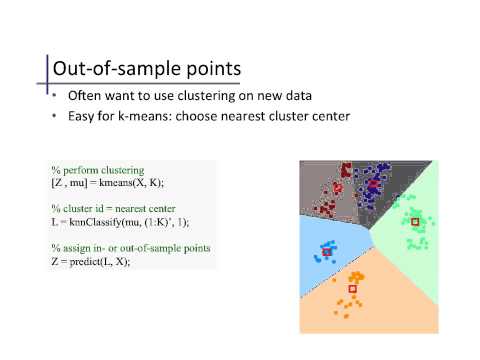
Once we have decided on the distance or similarity function we can decide a number of cluster centers, $K$. We find their location by allocating each center to a sub-set of the points and minimizing the sum of the squared errors,

\[E(\mathbf{M}) = \sum_{i \in \mathbf{i}_j} (\mathbf{x}_i - \mathbf{m}_j)^2,\]

where the notation $\mathbf{i}_j$ represents all the indices of each data point which has been allocated to the $j$th cluster represented by the center $\mathbf{m}_j$.

$k$-Means Clustering

One approach to minimizing this objective function is known as $k$-means clustering. It is simple and relatively quick to implement, but it is an initialization sensitive algorithm. Initialization is the process of choosing an initial set of parameters before optimization. For $k$-means clustering you need to choose an initial set of centers. In $k$-means clustering your final set of clusters is very sensitive to the initial choice of centers. For more technical details on $k$-means clustering you can watch a video of Alex Ihler introducing the algorithm here.

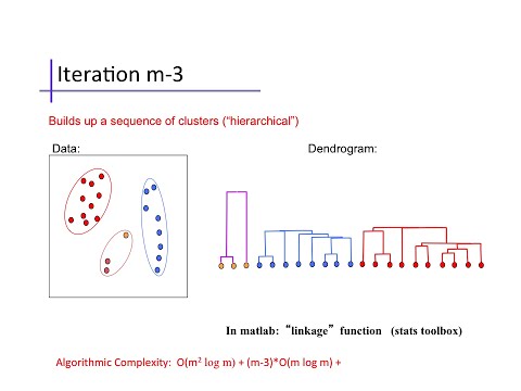
Hierarchical Clustering

Other approaches to clustering involve forming taxonomies of the cluster centers, like humans apply to animals, to form trees. You can learn more about agglomerative clustering in this video from Alex Ihler

Indeed one application of machine learning techniques is performing a hierarchical clustering based on genetic data, i.e. the actual contents of the genome. If we do this across a number of species then we can produce a phylogeny. The phylogeny aims to represent the actual evolution of the species and some phylogenies even estimate the timing of the common ancestor between two species³. Similar methods are used to estimate the origin of viruses like AIDS or Bird flu which mutate very quickly. Determining the origin of viruses can be important in containing or treating outbreaks.

An e-commerce company could apply hierarchical clustering to all its products. That would give a phylogeny of products. Each cluster of products would be split into sub-clusters of products until we got down to individual products. For example we might expect a high level split to be Electronics/Clothing. Of course, a challenge with these tree like structures is that many products belong in more than one parent cluster: for example running shoes should be in more than one group, they are ‘sporting goods’ and they are ‘apparel’. A tree structure doesn’t allow this allocation.

Our own psychological grouping capabilities are studied as a domain of cognitive science. Researchers like Josh Tenenbaum have developed algorithms that decompose data in more complex ways, but they can normally only be applied to smaller data sets.

Dimensionality Reduction

Dimensionality reduction methods compress the data by replacing the original data with a reduced number of continuous variables. One way of thinking of these methods is to imagine a marionette.

Thinking of dimensionality reduction as a marionette. We observe the high dimensional pose of the puppet, $\mathbf{x}$, but the movement of the puppeteer’s hand, $\mathbf{z}$ remains hidden to us. Dimensionality reduction aims to recover those hidden movements which generated the observations.

The position of each body part of a marionette could be thought of as our data, $\mathbf{x}_i$. So each data point consists of the 3-D co-ordinates of all the different body parts of the marionette. Lets say there are 13 different body parts (2 each of feet, knees, hips, hands, elbows, shoulders, one head). Each body part has an x, y, z position in Cartesian coordinates. So that’s 39 numbers associated with each observation.

The movement of these 39 parts is determined by the puppeteer via strings. Let’s assume it’s a very simple puppet, with just one stick to control it. The puppeteer can move the stick up and down, left and right. And they can twist it. This gives three parameters in the puppeteers control. This implies that the 39 variables we see moving are controlled by only 3 variables. These 3 variables are often called the hidden or latent variables.

Dimensionality reduction assumes something similar for real world data. It assumes that the data we observe is generated from some lower dimensional underlying process. It then seeks to recover the values associated with this low dimensional process.

Dimensionality reduction techniques underpin a lot of psychological scoring tests such as IQ tests or personality tests. An IQ test can involve several hundred questions, potentially giving a rich, high dimensional, characterization of some aspects of your intelligence. It is then summarized by a single number. Similarly the Myers-Briggs personality test involves answering

These tests are assuming that our intelligence is implicitly one dimensional and that our personality is implicitly four dimensional. Other examples include political belief which is typically represented on a left to right scale. A one dimensional distillation of an entire philosophy about how a country should be run. Our own leadership principles imply that our decisions have a fourteen dimensional space underlying them. Each decision could be characterized by judging to what extent it embodies each of the principles.

Political belief, personality, intelligence, leadership. None of these exist as a directly measurable quantity in the real world, rather they are inferred based on measurables. Dimensionality reduction is the process of allowing the computer to automatically find such underlying dimensions. This automatically allowing us to characterize each data point according to those explanatory variables. Neil is intelligent, moderately left wing extrovert who prefers rational thinking to feeling. His leadership decisions often exhibit ownership and backbone, but could don’t score highly on frugality. Each of these characteristics can be scored, and individuals can then be turned into vectors.

This doesn’t only apply to individuals, in recent years work on language modeling has taken a similar approach to words. The word2vec algorithm performed a dimensionality reduction on words, now you can take any word and map it to a latent space where similar words exhibit similar characteristics. A personality space for words.

Principal Component Analysis

Principal component analysis (PCA) is arguably the queen of dimensionality reduction techniques. PCA was developed as an approach to dimensionality reduction in 1930s by Hotelling as a method for the social sciences. In Hotelling’s formulation of PCA it was assumed that any data point, $\mathbf{x}$ could be represented as a weighted sum of the latent factors of interest, so that Hotelling described prediction functions (like in regression and classification above), only the regression is now multiple output. And instead of predicting a label, $y_i$, we now try and force the regression to predict the observed feature vector, $\mathbf{x}_i$. So for example, on an IQ test we would try and predict subject $i$’s answer to the $j$th question with the following function \(x_{ij} = f_j(z_i; \mathbf{w}).\) Here $z_i$ would be the IQ of subject $i$ and $f_j(\cdot)$ would be a function representing the relationship between the subject’s IQ and their score on the answer to question $j$. This function is the same for all subjects, but the subject’s IQ is assumed to differ leading to different scores for each subject.

Visualization of the first two principal components of an artificial data set. The data was generated by taking an image of a handwritten digit, 6, and rotating it 360 times, one degree each time. The first two principal components have been extracted in the diagram. The underlying circular shape is derived from the rotation of the data. Each image in the data set is projected on to the location its projected to in the latent space.

In Hotelling’s formulation he assumed that the function was a linear function. This idea is taken from a wider field known as factor analysis, so Hotelling described the challenge as

\[f_j(z_i; \mathbf{w}) = w_j z_i\]

so the answer to the $j$th question is predicted to be a scaling of the subject’s IQ. The scale factor is given by $w_j$. If there are more latent dimensions then a matrix of parameters, $\mathbf{W}$ is used, for example if there were two latent dimensions we’d have

\[f_j(\mathbf{z}_i; \mathbf{W}) = w_{1j} z_{1i} + w_{2j} z_{2i},\]

where, if this were a personality test, then $z_{1i}$ might represent the spectrum over a subject’s extrovert/introvert and $z_{2i}$ might represent where the subject was on the rational/perceptual scale. The function would make a prediction about the subjects answer to a particular question on the test (e.g. preference for office job vs preference for outdoor job). In factor analysis the parameters $\mathbf{W}$ are known as the factor loadings and in PCA they are known as the principal components.

Fitting the model involves finding estimates for the loadings, $\mathbf{W}$, and latent variables, $\mathbf{Z}$. There are different approaches including least squares. The least squares approach is used, for example, in recommender systems. In recommender systems this method is called matrix factorization. The the customer characteristics, $\mathbf{x}_i$ is the customer rating for each different product (or item) and the latent variables can be seen as a space of customer preferences. In the recommender system case the loadings matrix also has an interpretation as product similarities.⁴ Recommender systems have a particular characteristic in that most of the entries of the vector $\mathbf{x}_i$ are missing most of the time.

In PCA and factor analysis the unknown latent factors are dealt with through a probability distribution. They are each assumed to be drawn from a zero mean, unit variance normal distribution. This leaves the factor loadings to be estimated. For PCA the maximum likelihood solution for the factor loadings can be shown to be given by the eigenvalue decomposition of the data covariance matrix. This is algorithmically simple and convenient, although slow to compute for very large data sets with many features and many subjects. The eigenvalue problem can also be derived from many other starting points: e.g. the directions of maximum variance in the data or finding a latent space that best preserves inter-point distances between the data, or the optimal linear compression of the data given a linear reconstruction. These many and varied justifications for the eigenvalue decomposition may account for the popularity of PCA. Indeed, there is even an interpretation for Google’s original PageRank algorithm (which computed the smallest eigenvector of the internet’s linkage matrix) as seeking the dominant principal component of the web.⁵

Characterizing users according to past buying behavior and combining this with characteristics about products, is key to making good recommendations and returning useful search results. Further advances can be made if we understand the context of a particular session. For example, if a user is buying Christmas presents and searches for a dress, then it could be the case that the user is willing to spend a little more on the dress than in normal circumstances. Characterizing these effects requires more data and more complex algorithms. However, in domains such a search we are normally constrained by the speed with which we need to return results. Accounting for each of these factors while returning results with acceptable latency is a particular challenge.

Reinforcement Learning

The final domain of learning we will review is known as reinforcement learning. The domain of reinforcement learning is one that many researchers seem to believe is offering a route to general intelligence. The idea of general intelligence is to develop algorithms that are adaptable to many different circumstances. Supervised learning algorithms are designed to resolve particular challenges. Data is annotated with those challenges in mind. Unsupervised attempts to build representations without any context. But normally the algorithm designer has an understanding of what the broader objective is and designs the algorithms accordingly (for example, characterizing users). In reinforcement learning some context is given, in the form of a reward, but the reward is normally delayed. There may have been many actions that affected the outcome, but which actions had a positive effect and which a negative effect?

One issue for many companies is that the best way of testing the customer experience, A/B testing, prioritizes short term reward. The internet is currently being driven by short term rewards which make it distracting in the short term, but perhaps less useful in the long term. Click-bait is an example, but there are more subtle effects. The success of Facebook is driven by its ability to draw us in when likely we should be doing something else. This is driven by large scale A/B testing.

One open question is how to drive non-visual interfaces through equivalents to A/B testing. Speech interfaces, such as those used in intelligent agents, are less amenable to A/B testing when determining the quality of the interface. Improving interaction with them is therefore less exact science than the visual interface. Data efficient reinforcement learning methods are likely to be key to improving these agent’s ability to interact with the user and understand intent. However, they are not yet mature enough to be deployed in this application.

An area where reinforcement learning methods have been deployed with high profile success is game play. In game play the reward is delayed to the end of the game, and it comes in the form of victory or defeat. A significant advantage of game play as an application area is that, through simulation of the game, it is possible to generate as much data as is required to solve the problem. For this reason, many of the recent advances in reinforcement learning have occurred with methods that are not data efficient.

The company DeepMind is set up around reinforcement learning as an approach to general intelligence. All their most well known achievements are centered around artificial intelligence in game play. In reinforcement learning a decision made at any given time have a downstream affect on the result. Whether the effect if beneficial or not is unknown until a future moment.

We can think of reinforcement learning as providing a label, but the label is associated with a series of data involving a number of decisions taken. Each decision was taken given the understanding of game play at any given moment. Understanding which of these decisions was important in victory or defeat is a hard problem.

In machine learning the process of understanding which decisions were beneficial and which were detrimental is known as the credit allocation problem. You wish to reward decisions that led to success to encourage them, but punish decisions that lead to failure.

Broadly speaking, DeepMind uses an approach to Machine Learning where there are two mathematical functions at work. One determines the action to be taken at any given moment, the other estimates the quality of the board position at any given time. These are respectively known as the policy network and the value network.⁶ DeepMind made use of convolutional neural networks for both these models.

The ancient Chinese game of Go was considered a challenge for artificial intelligence for two reasons. Firstly, the game tree has a very high branching factor. The game tree is a discrete representation of the game. Every node in the game tree is associated with a board position. You can move through the game tree by making legal a move on the board to change the position. In Go, there are so many legal moves that the game tree increases exponentially. This challenge in Go was addressed by using stochastic game tree search. Rather than exploring the game tree exhaustively they explored it randomly.

Secondly, evaluating the quality of any given board position was deemed to be very hard.⁷ The value function determines for each player whether they are winning or loosing. Skilled Go players can assess a board position, but they do it by instinct, by intuition. Just as early AI researchers struggled to give rules for detecting cancer, it is challenging to give rules to assess a Go board. The machine learning approach that AlphaGo took is to train a value function network to make this assessment.

Reinforcement Learning and Classical Control

The approach that DeepMind took to conquering Go is a model free approach known as Q-learning.⁶ The model free approach refers to the fact that they don’t directly include a model of how the world evolves in the reinforcement learning algorithm. They make extensive use of the game tree, but they don’t model how it evolves. They do model the expected reward of each position in the game tree (the value function) but that is not the same as modeling how the game will proceed.

An alternative approach to reinforcement learning is to use a prediction function to suggest how the world will evolve in response to your actions. To predict how the game tree will evolve. You can then use this prediction to indirectly infer the expected reward associated with any action. This is known as model based reinforcement learning.

This model based approach is also closer to a control system. A classical control system is one where you give the system a set point. For example, a thermostat in the house. You set the temperature and the boiler switches off when it reaches it. Optimal control is about getting the house to the right temperature as quickly as possible. Classical control is widely used in robotic control and flight control.

One interesting crossover between classical control and machine learning arises because classical optimal control can be seen as a form of model based reinforcement learning. One where the reward is recovered when the set point is reached. In control engineering the prediction function is known as the transfer function. The process of fitting the transfer function in control is known as system identification.

There is some exciting work emerging at the interface between the areas of control and reinforcement learning. Results at this interface could be very important for improving the quality of robotic and drone control.

Optimization Methods

As we implied above, reinforcement learning can also used to improve user experience. In that case the reward is gained when the user buys a product from us. This makes it closely allied to the area of optimization. Optimization of our user interfaces can be seen as a reinforcement learning task, but more commonly it is thought about separately in the domains of Bayesian optimization or bandit learning.

We use optimization in machine learning to find the parameters of our models. We can do that because we have a mathematical representation of our objective function as a direct function of the parameters.

Examples in this form of optimization include, what is the best user interface for presenting adverts? What is the best design for a front wing for an F1 racing car? Which product should I return top of the list in response to this user’s search?

Bayesian optimization arises when we can’t directly relate the parameters in the system of interest to our objective through a mathematical function. For example, what is the mathematical function that relates a user’s experience to the probability that they will buy a product?

Bayesian Optimization

One approach to these problems is to use machine learning methods to develop a surrogate model for the optimization task. The surrogate model is a prediction function that attempts to recreate the process we are finding hard to model. We try to simultaneously fit the surrogate model and optimize the process.

Bayesian optimization methods use a surrogate model (normally a specific form of regression model). They use this to predict how the real system will perform. The surrogate model makes a prediction (with an estimate of the uncertainty) of what the response will be to any given input. Parameters to test are chosen by considering this prediction. Similar to reinforcement learning, this can be viewed as a model based approach because the surrogate model can be seen as a model of the real world. In bandit methods strategies are determined without turning to a model to motivate them. They are model free methods.

Model Based and Model Free: Performance

Because of their different philosophies, if a class of prediction functions is chosen, then a model based approach might have better average case performance. At least in terms of data efficiency. A model free approach may well have better worst case performance though, because it makes less assumptions about the nature of the data. To put it another way, making assumptions about the data is helpful if they are right: and if the model is sensible they’ll be right on average. However, it is unhelpful if the model is wrong. Indeed, it could be actively damaging. Since we can’t usually guarantee the model is absolutely right, the worst case performance of a model based approach would be poor.

Conclusion

We have introduced a range of machine learning approaches by focusing on their use of mathematical functions to replace manually coded systems of rules. The important characteristic of machine learning is that the form of these functions, as dictated by their parameters, is determined by acquiring data from the real world.

Deployment

The methods we have introduced are roughly speaking introduced in order of difficulty of deployment. While supervised learning is more involved in terms of collection of data, it is the most straightforward method to deploy once that data is recovered. For this reason, a major focus with supervised learning should always be on maintaining data quality, increasing the efficiency and accountability⁸ of the data collection pipeline and the quality of features used.

In relation to what AI can and can’t do today Andrew Ng is quoted as saying:

If a typical person can do a mental task with less than one second of thought, we can probably automate it using AI either now or in the near future.⁹

I would broadly agree with this quote but only in the context of supervised learning. If a human expert takes around that amount of time, then it’s also likely we can acquire the data necessary to build a supervised learning algorithm that can emulate that human’s response.

The picture with regard to unsupervised learning and reinforcement learning is more clouded.

One observation is that for supervised learning we seem to be moving beyond the era where very deep machine learning expertise is required to deploy methods. A solid understanding of machine learning (say to Masters level) is certainly required, but the quality of the final result is likely more dependent on domain expertise and the quality of the data and the information processing pipeline. This seems part of a wider trend where some of the big successes in machine learning are moving rapidly from the domain of science to that of engineering.¹⁰

So if we can only emulate tasks that humans take around a second to do, how are we managing to deliver on self driving cars? The answer is that we are constructing engineered systems from sub-components, each of which is a machine learning subsystem. But they are tied together as a component based system in line with our traditional engineering approach. This has an advantage that each component in the system can be verified before its inclusion. This is important for debugging and safety. But in practice we can expect these systems to be very brittle. A human adapts the way in which they drive the car across their lifetime. A human can react to other road users. In extreme situations, such as a car jacking, a human can set to one side normal patterns of behavior, and purposely crash their car to draw attention to the situation.

Supervised machine learning solutions are normally trained offline. They do not adapt when deployed because this makes them less verifiable. But this compounds the brittleness of our solutions. By deploying our solutions we actually change the environment in which they operate. Therefore, it’s important that they can be quickly updated to reflect changing circumstances. This updating happens offline. For a complex mechanical system, such as a delivery drone, extensive testing of the system may be required when any component is updated. It is therefore imperative that these data processing pipelines are well documented so that they can be redeployed on demand.

In practice there can be challenges with the false dichotomy between reproducibility and performance. It is likely that most of our data scientists are caring less about their ability to redeploy their pipelines and only about their ability to produce an algorithm that achieves a particular performance. A key question is how reproducible is that process? There is a false dichotomy because ensuring reproducibility will typically improve performance as it will make it easier to run a rigorous set of explorative experiments. A worry is that, currently, we do not have a way to quantify the scale of this potential problem within companies.

Common to all machine learning methods is the initial choice of useful classes of functions. The deep learning revolution is associated with a particular class of mathematical functions that is proving very successful in what were seen to be challenging domains: speech, vision, language. This has meant that significant advances in problems that have been seen as hard have occurred in artificial intelligence.