Abstract

Processing of personally sensitive information should respect an individual’s privacy. One promising framework is Differential Privacy (DP). In this talk I’ll present work led by Michael Smith at the University of Sheffield on the use of cloaking functions to make Gaussian process (GP) predictions differentially private. Gaussian process models are flexible models with particular advantages in handling missing and noisy data. Our hope is that advances in DP for GPs will make it easier to ‘learn without looking,’ i.e. gain the advantages of prediction from patient data without impinging on their privacy.

Joint work with Michael T. Smith, Max Zwiessele and Mauricio Alvarez

Embodiment Factors

bits/min	billions	2,000
billion calculations/s	~100	a billion
embodiment	20 minutes	5 billion years

Figure: Embodiment factors are the ratio between our ability to compute and our ability to communicate. Relative to the machine we are also locked in. In the table we represent embodiment as the length of time it would take to communicate one second’s worth of computation. For computers it is a matter of minutes, but for a human, it is a matter of thousands of millions of years. See also “Living Together: Mind and Machine Intelligence” Lawrence (2017)

There is a fundamental limit placed on our intelligence based on our ability to communicate. Claude Shannon founded the field of information theory. The clever part of this theory is it allows us to separate our measurement of information from what the information pertains to.¹

Shannon measured information in bits. One bit of information is the amount of information I pass to you when I give you the result of a coin toss. Shannon was also interested in the amount of information in the English language. He estimated that on average a word in the English language contains 12 bits of information.

Given typical speaking rates, that gives us an estimate of our ability to communicate of around 100 bits per second (Reed and Durlach, 1998). Computers on the other hand can communicate much more rapidly. Current wired network speeds are around a billion bits per second, ten million times faster.

When it comes to compute though, our best estimates indicate our computers are slower. A typical modern computer can process make around 100 billion floating point operations per second, each floating point operation involves a 64 bit number. So the computer is processing around 6,400 billion bits per second.

It’s difficult to get similar estimates for humans, but by some estimates the amount of compute we would require to simulate a human brain is equivalent to that in the UK’s fastest computer (Ananthanarayanan et al., 2009), the MET office machine in Exeter, which in 2018 ranks as the 11th fastest computer in the world. That machine simulates the world’s weather each morning, and then simulates the world’s climate in the afternoon. It is a 16 petaflop machine, processing around 1,000 trillion bits per second.

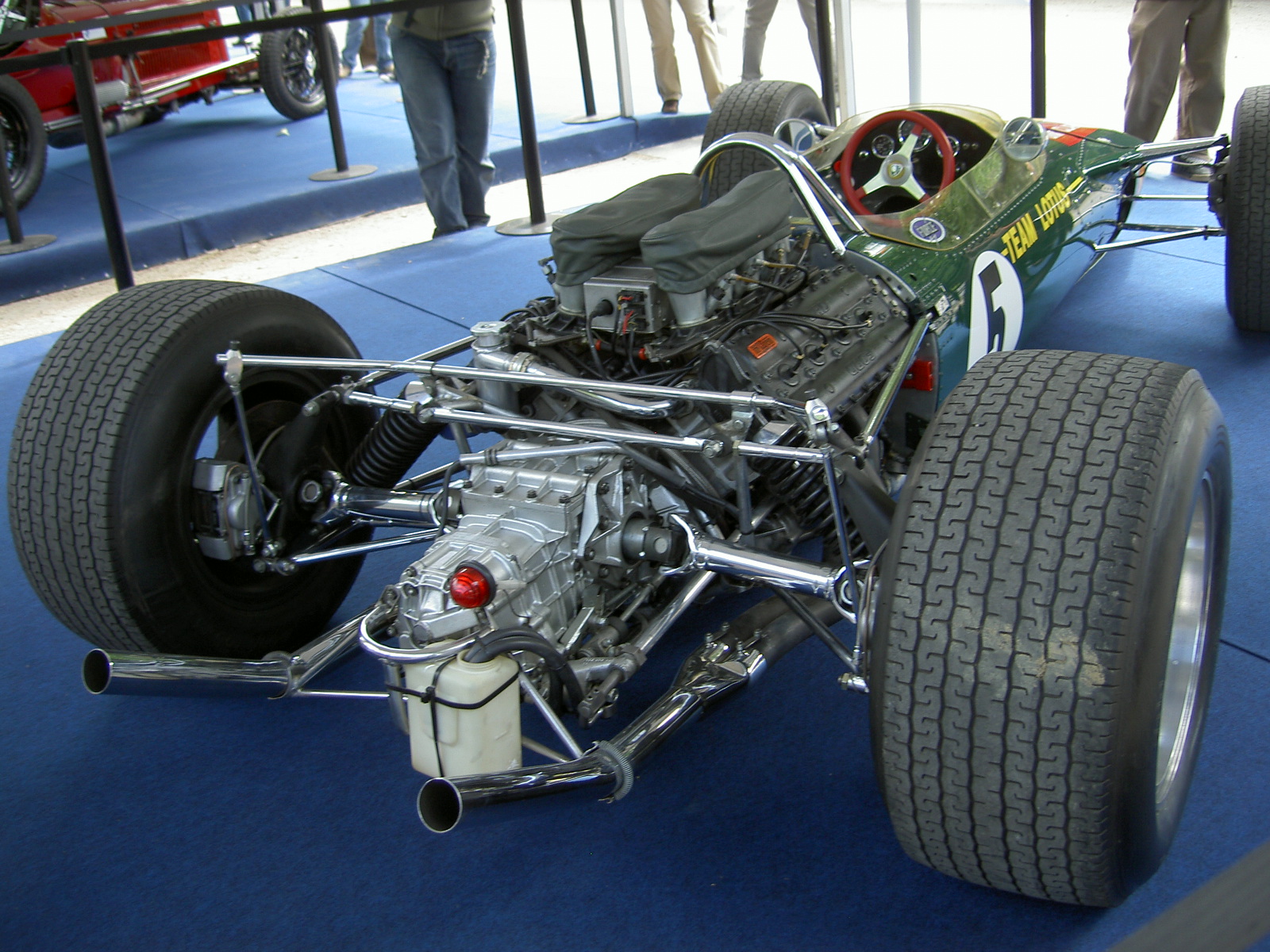
Figure: The Lotus 49, view from the rear. The Lotus 49 was one of the last Formula One cars before the introduction of aerodynamic aids.

So when it comes to our ability to compute we are extraordinary, not compute in our conscious mind, but the underlying neuron firings that underpin both our consciousness, our subconsciousness as well as our motor control etc.

If we think of ourselves as vehicles, then we are massively overpowered. Our ability to generate derived information from raw fuel is extraordinary. Intellectually we have formula one engines.

But in terms of our ability to deploy that computation in actual use, to share the results of what we have inferred, we are very limited. So when you imagine the F1 car that represents a psyche, think of an F1 car with bicycle wheels.

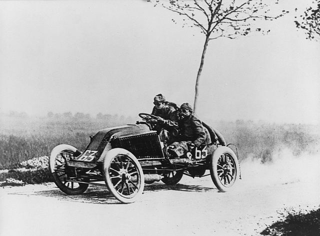
Figure: Marcel Renault races a Renault 40 cv during the Paris-Madrid race, an early Grand Prix, in 1903. Marcel died later in the race after missing a warning flag for a sharp corner at Couhé Vérac, likely due to dust reducing visibility.

Just think of the control a driver would have to have to deploy such power through such a narrow channel of traction. That is the beauty and the skill of the human mind.

In contrast, our computers are more like go-karts. Underpowered, but with well-matched tires. They can communicate far more fluidly. They are more efficient, but somehow less extraordinary, less beautiful.

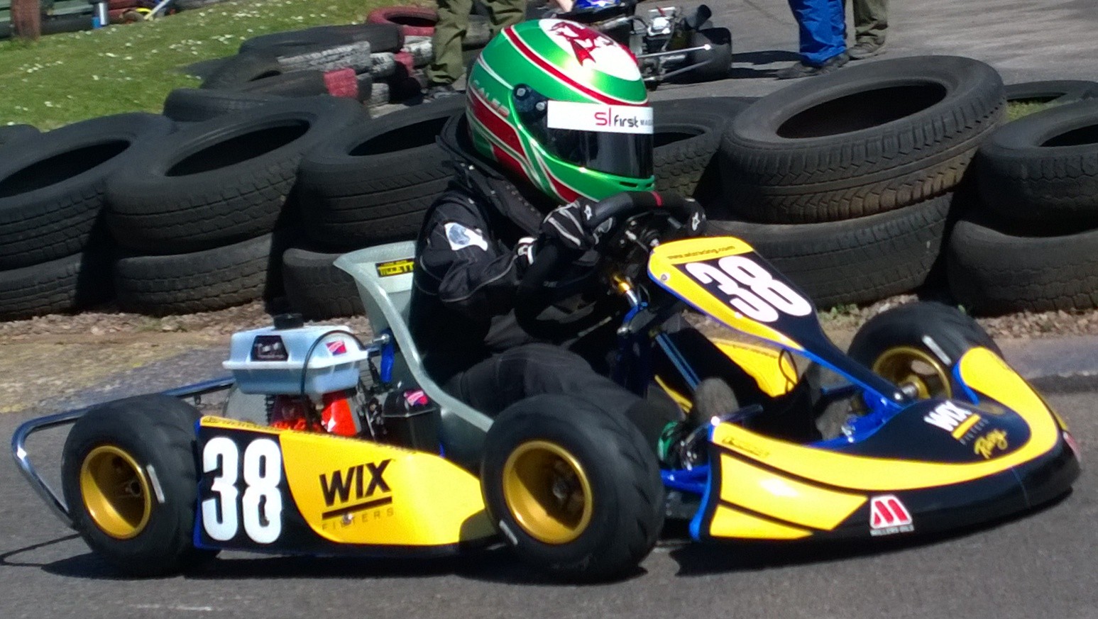
Figure: Caleb McDuff driving for WIX Silence Racing.

For humans, that means much of our computation should be dedicated to considering what we should compute. To do that efficiently we need to model the world around us. The most complex thing in the world around us is other humans. So it is no surprise that we model them. We second guess what their intentions are, and our communication is only necessary when they are departing from how we model them. Naturally, for this to work well, we need to understand those we work closely with. So it is no surprise that social communication, social bonding, forms so much of a part of our use of our limited bandwidth.

There is a second effect here, our need to anthropomorphise objects around us. Our tendency to model our fellow humans extends to when we interact with other entities in our environment. To our pets as well as inanimate objects around us, such as computers or even our cars. This tendency to over interpret could be a consequence of our limited ability to communicate.²

For more details see this paper “Living Together: Mind and Machine Intelligence”, and this TEDx talk.

Evolved Relationship with Information

The high bandwidth of computers has resulted in a close relationship between the computer and data. Large amounts of information can flow between the two. The degree to which the computer is mediating our relationship with data means that we should consider it an intermediary.

Originaly our low bandwith relationship with data was affected by two characteristics. Firstly, our tendency to over-interpret driven by our need to extract as much knowledge from our low bandwidth information channel as possible. Secondly, by our improved understanding of the domain of mathematical statistics and how our cognitive biases can mislead us.

With this new set up there is a potential for assimilating far more information via the computer, but the computer can present this to us in various ways. If it’s motives are not aligned with ours then it can misrepresent the information. This needn’t be nefarious it can be simply as a result of the computer pursuing a different objective from us. For example, if the computer is aiming to maximize our interaction time that may be a different objective from ours which may be to summarize information in a representative manner in the shortest possible length of time.

For example, for me, it was a common experience to pick up my telephone with the intention of checking when my next appointment was, but to soon find myself distracted by another application on the phone, and end up reading something on the internet. By the time I’d finished reading, I would often have forgotten the reason I picked up my phone in the first place.

There are great benefits to be had from the huge amount of information we can unlock from this evolved relationship between us and data. In biology, large scale data sharing has been driven by a revolution in genomic, transcriptomic and epigenomic measurement. The improved inferences that can be drawn through summarizing data by computer have fundamentally changed the nature of biological science, now this phenomenon is also infuencing us in our daily lives as data measured by happenstance is increasingly used to characterize us.

Better mediation of this flow actually requires a better understanding of human-computer interaction. This in turn involves understanding our own intelligence better, what its cognitive biases are and how these might mislead us.

For further thoughts see Guardian article on marketing in the internet era from 2015.

You can also check my blog post on System Zero. also from 2015.

New Flow of Information

Classically the field of statistics focussed on mediating the relationship between the machine and the human. Our limited bandwidth of communication means we tend to over-interpret the limited information that we are given, in the extreme we assign motives and desires to inanimate objects (a process known as anthropomorphizing). Much of mathematical statistics was developed to help temper this tendency and understand when we are valid in drawing conclusions from data.

Figure: The trinity of human, data and computer, and highlights the modern phenomenon. The communication channel between computer and data now has an extremely high bandwidth. The channel between human and computer and the channel between data and human is narrow. New direction of information flow, information is reaching us mediated by the computer. The focus on classical statistics reflected the importance of the direct communication between human and data. The modern challenges of data science emerge when that relationship is being mediated by the machine.

Data science brings new challenges. In particular, there is a very large bandwidth connection between the machine and data. This means that our relationship with data is now commonly being mediated by the machine. Whether this is in the acquisition of new data, which now happens by happenstance rather than with purpose, or the interpretation of that data where we are increasingly relying on machines to summarise what the data contains. This is leading to the emerging field of data science, which must not only deal with the same challenges that mathematical statistics faced in tempering our tendency to over interpret data, but must also deal with the possibility that the machine has either inadvertently or malisciously misrepresented the underlying data.

Bandwidth Constrained Conversations

Figure: Conversation relies on internal models of other individuals.

Figure: Misunderstanding of context and who we are talking to leads to arguments.

Embodiment factors imply that, in our communication between humans, what is not said is, perhaps, more important than what is said. To communicate with each other we need to have a model of who each of us are.

To aid this, in society, we are required to perform roles. Whether as a parent, a teacher, an employee or a boss. Each of these roles requires that we conform to certain standards of behaviour to facilitate communication between ourselves.

Control of self is vitally important to these communications.

The high availability of data available to humans undermines human-to-human communication channels by providing new routes to undermining our control of self.

Figure: A key reference for Gaussian process models remains the excellent book “Gaussian Processes for Machine Learning” (Rasmussen and Williams (2006)). The book is also freely available online.

Rasmussen and Williams (2006) is still one of the most important references on Gaussian process models. It is available freely online.

Bayesian Inference by Rejection Sampling

One view of Bayesian inference is to assume we are given a mechanism for generating samples, where we assume that mechanism is representing an accurate view on the way we believe the world works.

This mechanism is known as our prior belief.

We combine our prior belief with our observations of the real world by discarding all those prior samples that are inconsistent with our observations. The likelihood defines mathematically what we mean by inconsistent with the observations. The higher the noise level in the likelihood, the looser the notion of consistent.

The samples that remain are samples from the posterior.

This approach to Bayesian inference is closely related to two sampling techniques known as rejection sampling and importance sampling. It is realized in practice in an approach known as approximate Bayesian computation (ABC) or likelihood-free inference.

In practice, the algorithm is often too slow to be practical, because most samples will be inconsistent with the observations and as a result the mechanism must be operated many times to obtain a few posterior samples.

However, in the Gaussian process case, when the likelihood also assumes Gaussian noise, we can operate this mechanism mathematically, and obtain the posterior density analytically. This is the benefit of Gaussian processes.

First, we will load in two python functions for computing the covariance function.

Next, we sample from a multivariate normal density (a multivariate Gaussian), using the covariance function as the covariance matrix.

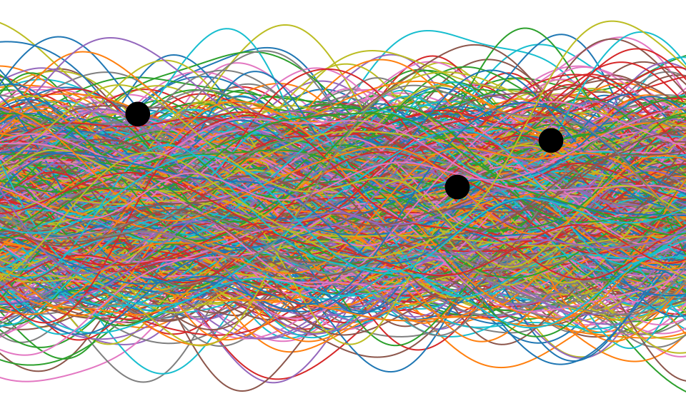
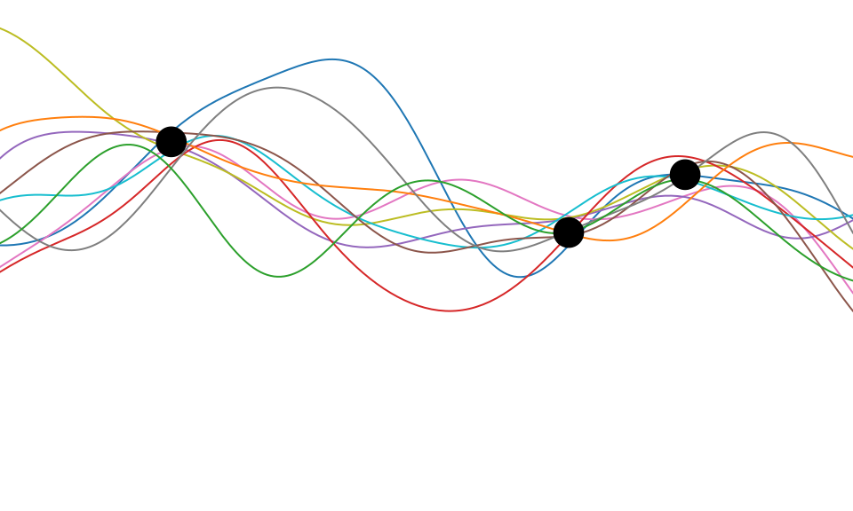
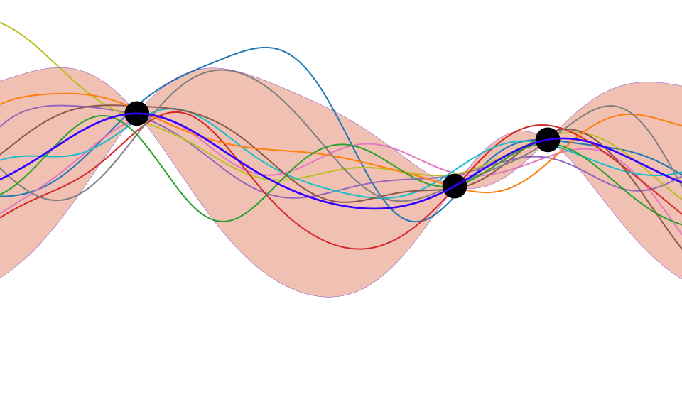
Figure: One view of Bayesian inference is we have a machine for generating samples (the prior), and we discard all samples inconsistent with our data, leaving the samples of interest (the posterior). This is a rejection sampling view of Bayesian inference. The Gaussian process allows us to do this analytically by multiplying the prior by the likelihood.

• We want to protect a user from a linkage attack…

  …while still performing inference over the whole group.

• Making a dataset private is more than just erasing names.

Narayanan and Felten (2014);Ohm (2010);Barth-Jones (2012)

• To achieve a level of privacy one needs to add randomness to the data.

• This is a fundamental feature of differential privacy.

See The Algorithmic Foundations of Differential Privacy by Dwork and Roth (2014) for a rigorous introduction to the framework.

Differential Privacy for Gaussian Processes

We have a dataset in which the inputs, \(\mathbf{X}\), are public. The outputs, \(\mathbf{ y}\), we want to keep private.

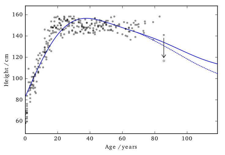
Data consists of the heights and weights of 287 women from a census of the !Kung (Howell, 1967)

Hall et al. (2013) showed that one can ensure that a version of \(f\), function \(\tilde{f}\) is \((\varepsilon, \delta)\)-differentially private by adding a scaled sample from a GP prior.

3 pages of maths ahead!

• We applied this method to the GP posterior.

• The covariance of the posterior only depends on the inputs, \(\mathbf{X}\). So we can compute this without applying DP.

• The mean function, \(f_D(\mathbf{ x}_*)\), does depend on \(\mathbf{ y}\). \[f_D(\mathbf{ x}_*) = \mathbf{ k}(x_*, \mathbf{X}) \mathbf{K}^{-1} \mathbf{ y}\]

• We are interested in finding

  \[|| f_D(\mathbf{ x}_*) - f_{D^\prime}(\mathbf{ x}_*) ||_H^2\]

  …how much the mean function (in RKHS) can change due to a change in \(\mathbf{ y}\).

• Using the representer theorem, we can write \[|| f_D(\mathbf{ x}_*) - f_{D^\prime}(\mathbf{ x}_*) ||_H^2\]

  as:

  \[\Big|\Big|\sum_{i=1}^nk(\mathbf{ x}_*,\mathbf{ x}_i) \left(\alpha_i - \alpha^\prime_i\right)\Big|\Big|_H^2\]

  where \(\boldsymbol{\alpha} - \boldsymbol{\alpha}^\prime = \mathbf{K}^{-1} \left(\mathbf{ y}- \mathbf{ y}^\prime \right)\)

• L2 Norm

  \[\Big|\Big|\sum_{i=1}^nk(\mathbf{ x}_*,\mathbf{ x}_i) \left(\alpha_i - \alpha^\prime_i\right)\Big|\Big|_H^2\]

  where \(\boldsymbol{\alpha} - \boldsymbol{\alpha}^\prime = \mathbf{K}^{-1} \left(\mathbf{ y}- \mathbf{ y}^\prime \right)\)

• We constrain the kernel: \(-1\leq k(\cdot,\cdot) \leq 1\) and we only allow one element of \(\mathbf{ y}\) and \(\mathbf{ y}^\prime\) to differ (by at most \(d\)).

• So only one column of \(\mathbf{K}^{-1}\) will be involved in the change of mean (which we are summing over).

• The distance above can then be shown to be no greater than \(d\;||\mathbf{K}^{-1}||_\infty\)

This ‘works’ in that it allows DP predictions…but to avoid too much noise, the value of \(\varepsilon\) is too large (here it is 100)

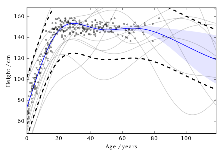
EQ kernel, \(\ell= 25\) years, \(\Delta=100\)cm

Using sparse methods (i.e. inducing inputs) can help reduce the sensitivity a little. We’ll see more on this later.

Cloaking

• So far we’ve made the whole posterior mean function private…

  …what if we just concentrate on making particular predictions private?

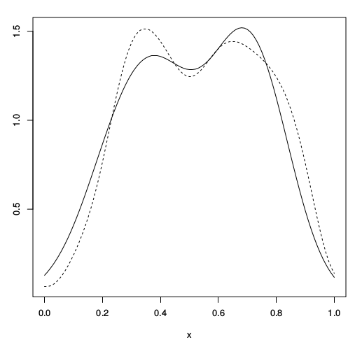
• Standard approach: sample the noise is from the GP’s prior.

• Not necessarily the most ‘efficient’ covariance to use.

Left: Function change. Right: test point change

Left: Function change. Right: test point change

Left: Function change. Right: test point change

Left: Function change. Right: test point change

Left: Function change. Right: test point change

Left: Function change. Right: test point change

• Hall et al. (2013) also presented a bound on vectors.

• Find a bound (\(\Delta\)) on the scale of the output change, in term of its Mahalanobis distance (wrt the added noise covariance).

  \[\sup_{D \sim {D^\prime}} ||\mathbf{M}^{-1/2} (\mathbf{ y}_* - \mathbf{ y}_{*}^\prime)||_2 \leq \Delta\]

• We use this to scale the noise we add:

  \[\frac{\text{c}(\delta)\Delta}{\varepsilon} \mathcal{N}_d(0,\mathbf{M})\]

  We get to pick \(\mathbf{M}\)

• Intuitively we want to construct \(\mathbf{M}\) so that it has greatest covariance in those directions most affected by changes in training points, so that it will be most able to mask those changes.

• The change in posterior mean predictions is,

  \[\mathbf{ y}_* - \mathbf{ y}^\prime_* = \mathbf{K}_{*f} \mathbf{K}^{-1} (\mathbf{ y}-\mathbf{ y}^\prime)\]

• Effect of perturbing each training point on each test point is represented in the cloaking matrix,

  \[\mathbf{C} = \mathbf{K}_{*f} \mathbf{K}^{-1}\]

• We assume we are protecting only one training input’s change, by at most \(d\).

• So \(\mathbf{ y}-\mathbf{ y}^\prime\) will be all zeros except for one element, \(i\).
  

• So the change in test points will be (at most)

  \[\mathbf{ y}_*^\prime - \mathbf{ y}_* = d \mathbf{C}_{:i}\]

• We’re able to write the earlier bound as,

  \[d^2 \sup_{i} \mathbf{c}_i^\top \mathbf{M}^{-1} \mathbf{c}_i \leq\Delta\]

  where \(\mathbf{c}_i \triangleq \mathbf{C}_{:i}\)

• Dealing with \(d\) elsewhere and setting \(\Delta = 1\) (thus \(0 \leq \mathbf{c}_i^\top \mathbf{M}^{-1} \mathbf{c}_i \leq 1\)) and minimise \(\log |\mathbf{M}|\) (minimises the partial entropy).

• Using Lagrange multipliers and gradient descent, we find \[ \mathbf{M} = \sum_i{\lambda_i \mathbf{c}_i \mathbf{c}_i^\top} \]

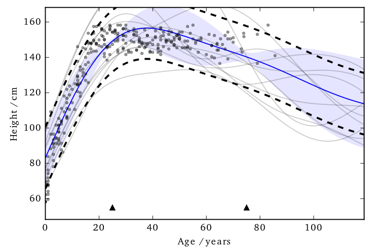
The noise added by this method is now practical.

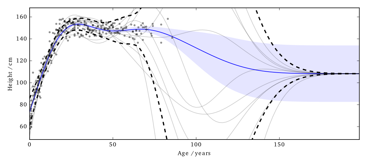
Figure:

EQ kernel, \(l = 25\) years, \(\Delta=100\)cm, \(\varepsilon=1\)

It also has some interesting features;

• Less noise where data is concentrated
• Least noise far from any data
• Most noise just outside data

Figure: Simple cloaking function.

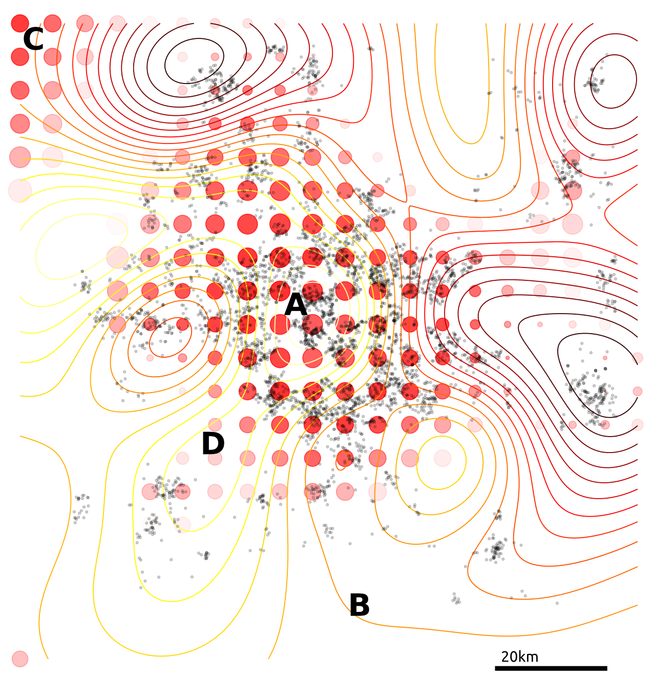
Figure: Simple cloaking function on house price data.

• Tested on 4D citibike dataset (predicting journey durations from start/finish station locations).

• The method appears to achieve lower noise than binning alternatives (for reasonable \(\varepsilon\)).

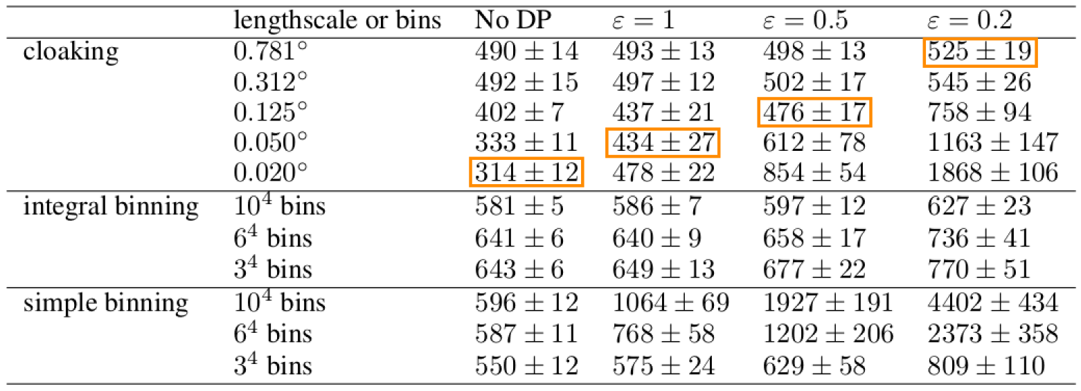
Figure: Citibike data. Lengthscale in degrees, values above, journey duration (in seconds).

• Outliers poorly predicted.

• Too much noise around data ‘edges.’

• Use inducing inputs to reduce the sensitivity to these outliers.

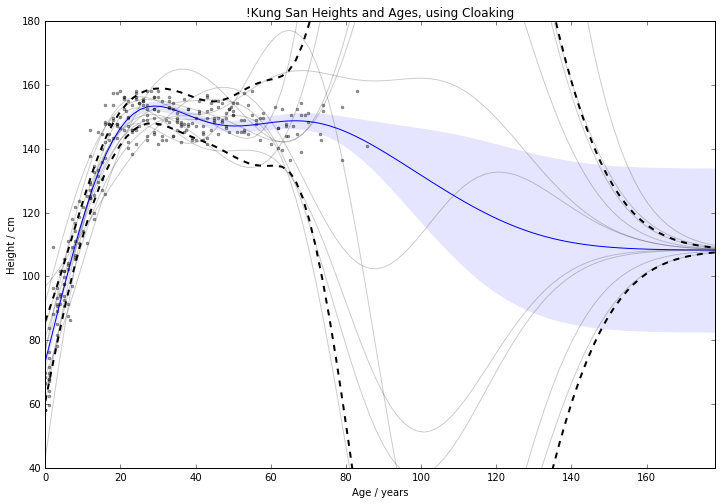
Figure: Cloaking function with no inducing inputs.

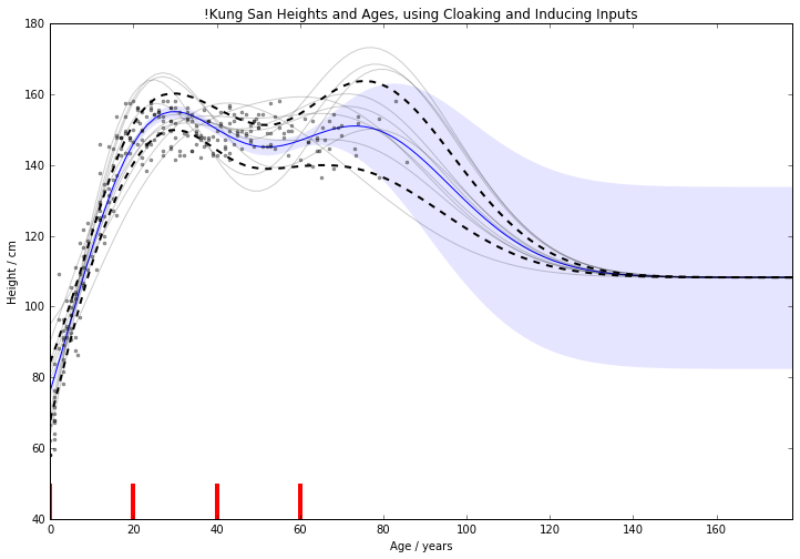
Figure: Cloaking function with inducing inputs.

• For 1D !Kung, RMSE improved from \(15.0 \pm 2.0 \text{cm}\) to \(11.1 \pm 0.8 \text{cm}\)

  Use Age and Weight to predict Height

• For 2D !Kung, RMSE improved from \(22.8 \pm 1.9 \text{cm}\) to \(8.8 \pm 0.6 \text{cm}\)

  Note that the uncertainty across cross-validation runs smaller. 2D version benefits from data’s 1D manifold.

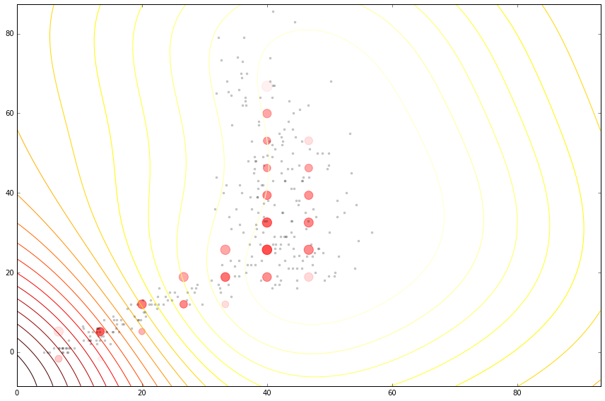
Figure: Cloaking functions on the housing data with no inducing inputs.

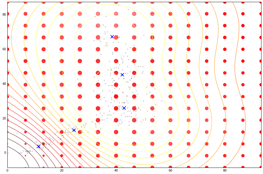
Figure: Cloaking functions on the housing data with inducing inputs.

• Summary We have developed an improved method for performing differentially private regression.

• Future work Multiple outputs, GP classification, DP Optimising hyperparameters, Making the inputs private.

• Thanks Funders: EPSRC; Colleagues: Michael T. Smith, Mauricio, Max.

• Recruiting Deep Probabilistic Models: 2 year postdoc (tinyurl.com/shefpostdoc)

Thanks!

For more information on these subjects and more you might want to check the following resources.

• twitter: @lawrennd

• podcast: The Talking Machines

• newspaper: Guardian Profile Page

• blog: http://inverseprobability.com

• Images used: BostonGlobe: Mass Mutual, Weld. Harvard: Sweeney. Rich on flickr: Sheffield skyline.

References

the challenge of understanding what information pertains to is known as knowledge representation.↩︎
Another related factor is our ability to store information. Mollica and Piantadosi (2019) suggest that during language acquisition we store 1.5 Megabytes of data (12 million bits). That would take around 2000 hours, or nearly twelve weeks, to transmit verbally.↩︎