Data First Culture
Abstract
Digital transformation has offered the promise of moving from a manual decision-making world to a world where decisions can be rational, data-driven and automated. The first step to digital transformation is mapping the world of atoms (material, customers, logistic networks) into the world of bits. But the real challenges may start once this is complete. In this talk we introduce the notion of ‘post digital transformation’: the challenges of doing business in a digital world.
Henry Ford’s Faster Horse


Figure: A 1925 Ford Model T built at Henry Ford’s Highland Park Plant in Dearborn, Michigan. This example now resides in Australia, owned by the founder of FordModelT.net. From https://commons.wikimedia.org/wiki/File:1925_Ford_Model_T_touring.jpg
It’s said that Henry Ford’s customers wanted a “a faster horse.” If Henry Ford was selling us artificial intelligence today, what would the customer call for, “a smarter human?” That’s certainly the picture of machine intelligence we find in science fiction narratives, but the reality of what we’ve developed is much more mundane.
Car engines produce prodigious power from petrol. Machine intelligences deliver decisions derived from data. In both cases the scale of consumption enables a speed of operation that is far beyond the capabilities of their natural counterparts. Unfettered energy consumption has consequences in the form of climate change. Does unbridled data consumption also have consequences for us?
If we devolve decision making to machines, we depend on those machines to accommodate our needs. If we don’t understand how those machines operate, we lose control over our destiny. Our mistake has been to see machine intelligence as a reflection of our intelligence. We cannot understand the smarter human without understanding the human. To understand the machine, we need to better understand ourselves.
Introduction
Setup
notutils
This small package is a helper package for various notebook utilities used
The software can be installed using
%pip install notutilsfrom the command prompt where you can access your python installation.
The code is also available on GitHub: https://github.com/lawrennd/notutils
Once notutils is installed, it can be imported in the usual manner.
import notutilspods
In Sheffield we created a suite of software tools for ‘Open Data Science.’ Open data science is an approach to sharing code, models and data that should make it easier for companies, health professionals and scientists to gain access to data science techniques.
You can also check this blog post on Open Data Science.
The software can be installed using
%pip install podsfrom the command prompt where you can access your python installation.
The code is also available on GitHub: https://github.com/lawrennd/ods
Once pods is installed, it can be imported in the usual manner.
import podsmlai
The mlai software is a suite of helper functions for teaching and demonstrating machine learning algorithms. It was first used in the Machine Learning and Adaptive Intelligence course in Sheffield in 2013.
The software can be installed using
%pip install mlaifrom the command prompt where you can access your python installation.
The code is also available on GitHub: https://github.com/lawrennd/mlai
Once mlai is installed, it can be imported in the usual manner.
import mlaiThe Gartner Hype Cycle
Figure: The Gartner Hype Cycle places technologies on a graph that relates to the expectations we have of a technology against its actual influence. Early hope for a new techology is often displaced by disillusionment due to the time it takes for a technology to be usefully deployed.
The Gartner Hype Cycle tries to assess where an idea is in terms of maturity and adoption. It splits the evolution of technology into a technological trigger, a peak of expectations followed by a trough of disillusionment and a final ascension into a useful technology. It looks rather like a classical control response to a final set point.
Cycle for ML Terms
Google Trends
%pip install pytrendsFigure: Google trends for ‘artificial intelligence,’ ‘big data,’ ‘data mining,’ ‘deep learning,’ ‘machine learning’ as different technological terms gives us insight into their popularity over time.
Google trends gives us insight into the interest for different terms over time.
Examining Google treds for ‘artificial intelligence,’ ‘big data,’ ‘data mining,’ ‘deep learning’ and ‘machine learning’ we can see that ‘artificial intelligence’ may be entering a plateau of productivity, ‘big data’ is entering the trough of disillusionment, and ‘data mining’ seems to be deeply within the trough. On the other hand, ‘deep learning’ and ‘machine learning’ appear to be ascending to the peak of inflated expectations having experienced a technology trigger.
For deep learning that technology trigger was the ImageNet result of 2012 (Krizhevsky et al., n.d.). This step change in performance on object detection in images was achieved through convolutional neural networks, popularly known as ‘deep learning.’
What is Machine Learning?
What is machine learning? At its most basic level machine learning is a combination of
\[\text{data} + \text{model} \stackrel{\text{compute}}{\rightarrow} \text{prediction}\]
where data is our observations. They can be actively or passively acquired (meta-data). The model contains our assumptions, based on previous experience. That experience can be other data, it can come from transfer learning, or it can merely be our beliefs about the regularities of the universe. In humans our models include our inductive biases. The prediction is an action to be taken or a categorization or a quality score. The reason that machine learning has become a mainstay of artificial intelligence is the importance of predictions in artificial intelligence. The data and the model are combined through computation.
In practice we normally perform machine learning using two functions. To combine data with a model we typically make use of:
a prediction function a function which is used to make the predictions. It includes our beliefs about the regularities of the universe, our assumptions about how the world works, e.g., smoothness, spatial similarities, temporal similarities.
an objective function a function which defines the cost of misprediction. Typically, it includes knowledge about the world’s generating processes (probabilistic objectives) or the costs we pay for mispredictions (empirical risk minimization).
The combination of data and model through the prediction function and the objective function leads to a learning algorithm. The class of prediction functions and objective functions we can make use of is restricted by the algorithms they lead to. If the prediction function or the objective function are too complex, then it can be difficult to find an appropriate learning algorithm. Much of the academic field of machine learning is the quest for new learning algorithms that allow us to bring different types of models and data together.
A useful reference for state of the art in machine learning is the UK Royal Society Report, Machine Learning: Power and Promise of Computers that Learn by Example.
You can also check my post blog post on What is Machine Learning?.
Artificial Intelligence and Data Science
Artificial intelligence has the objective of endowing computers with human-like intelligent capabilities. For example, understanding an image (computer vision) or the contents of some speech (speech recognition), the meaning of a sentence (natural language processing) or the translation of a sentence (machine translation).
Supervised Learning for AI
The machine learning approach to artificial intelligence is to collect and annotate a large data set from humans. The problem is characterized by input data (e.g. a particular image) and a label (e.g. is there a car in the image yes/no). The machine learning algorithm fits a mathematical function (I call this the prediction function) to map from the input image to the label. The parameters of the prediction function are set by minimizing an error between the function’s predictions and the true data. This mathematical function that encapsulates this error is known as the objective function.
This approach to machine learning is known as supervised learning. Various approaches to supervised learning use different prediction functions, objective functions or different optimization algorithms to fit them.
For example, deep learning makes use of neural networks to form the predictions. A neural network is a particular type of mathematical function that allows the algorithm designer to introduce invariances into the function.
An invariance is an important way of including prior understanding in a machine learning model. For example, in an image, a car is still a car regardless of whether it’s in the upper left or lower right corner of the image. This is known as translation invariance. A neural network encodes translation invariance in convolutional layers. Convolutional neural networks are widely used in image recognition tasks.
An alternative structure is known as a recurrent neural network (RNN). RNNs neural networks encode temporal structure. They use auto regressive connections in their hidden layers, they can be seen as time series models which have non-linear auto-regressive basis functions. They are widely used in speech recognition and machine translation.
Machine learning has been deployed in Speech Recognition (e.g. Alexa, deep neural networks, convolutional neural networks for speech recognition), in computer vision (e.g. Amazon Go, convolutional neural networks for person recognition and pose detection).
The field of data science is related to AI, but philosophically different. It arises because we are increasingly creating large amounts of data through happenstance rather than active collection. In the modern era data is laid down by almost all our activities. The objective of data science is to extract insights from this data.
Classically, in the field of statistics, data analysis proceeds by assuming that the question (or scientific hypothesis) comes before the data is created. E.g., if I want to determine the effectiveness of a particular drug, I perform a design for my data collection. I use foundational approaches such as randomization to account for confounders. This made a lot of sense in an era where data had to be actively collected. The reduction in cost of data collection and storage now means that many data sets are available which weren’t collected with a particular question in mind. This is a challenge because bias in the way data was acquired can corrupt the insights we derive. We can perform randomized control trials (or A/B tests) to verify our conclusions, but the opportunity is to use data science techniques to better guide our question selection or even answer a question without the expense of a full randomized control trial (referred to as A/B testing in modern internet parlance).
Intellectual Debt
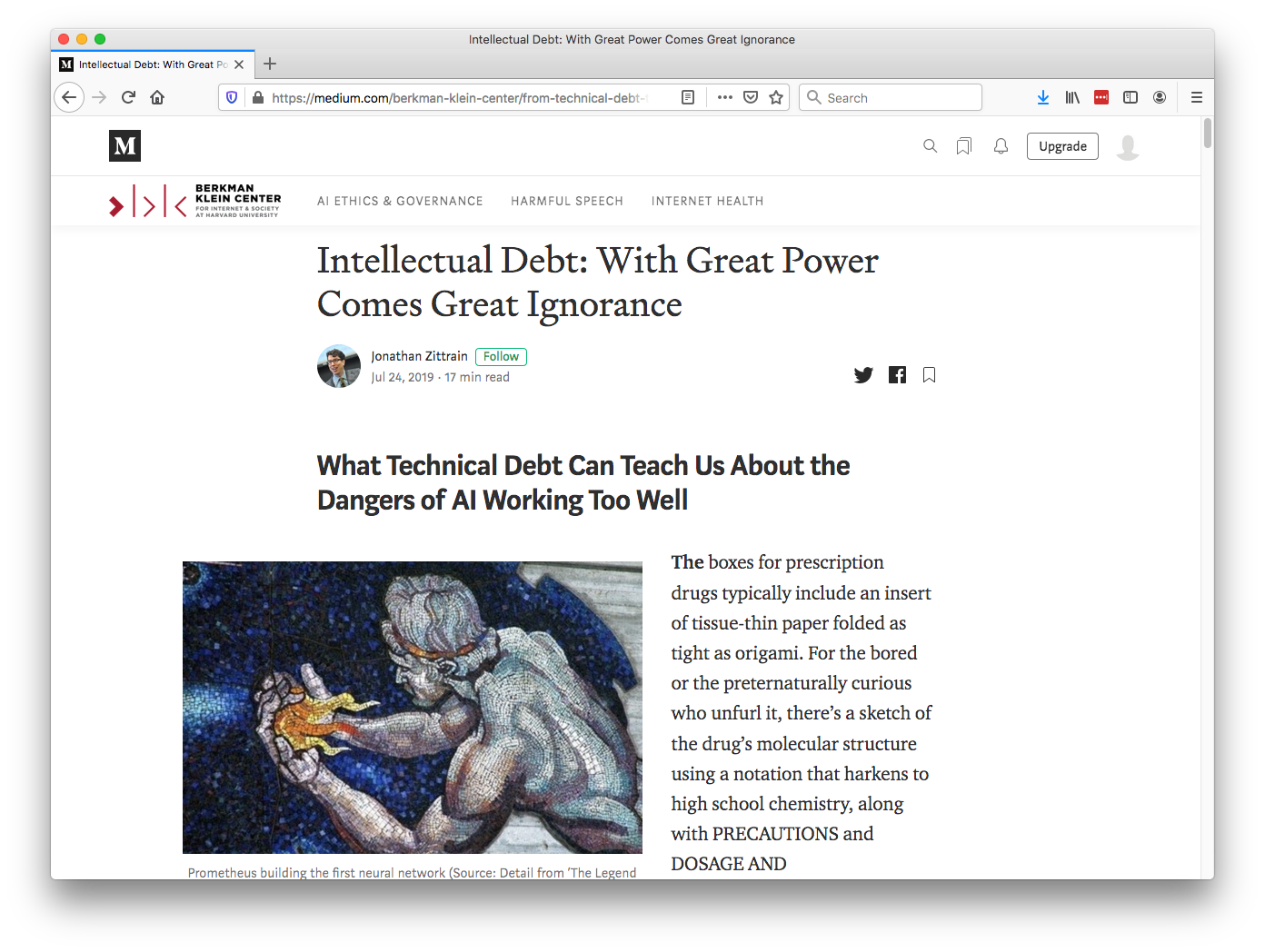
Figure: Jonathan Zittrain’s term to describe the challenges of explanation that come with AI is Intellectual Debt.
Information and Embodiment
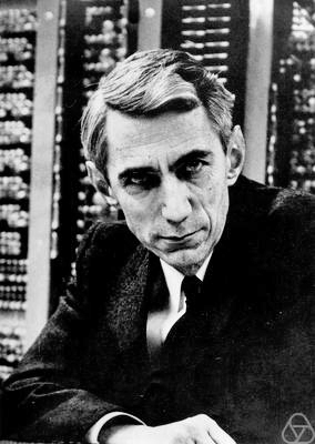
Figure: Claude Shannon (1916-2001)
| bits/min | billions | 2,000 |
|
billion calculations/s |
~100 | a billion |
| embodiment | 20 minutes | 5 billion years |
Figure: Embodiment factors are the ratio between our ability to compute and our ability to communicate. Relative to the machine we are also locked in. In the table we represent embodiment as the length of time it would take to communicate one second’s worth of computation. For computers it is a matter of minutes, but for a human, it is a matter of thousands of millions of years.
Evolved Relationship with Information
The high bandwidth of computers has resulted in a close relationship between the computer and data. Large amounts of information can flow between the two. The degree to which the computer is mediating our relationship with data means that we should consider it an intermediary.
Originaly our low bandwith relationship with data was affected by two characteristics. Firstly, our tendency to over-interpret driven by our need to extract as much knowledge from our low bandwidth information channel as possible. Secondly, by our improved understanding of the domain of mathematical statistics and how our cognitive biases can mislead us.
With this new set up there is a potential for assimilating far more information via the computer, but the computer can present this to us in various ways. If it’s motives are not aligned with ours then it can misrepresent the information. This needn’t be nefarious it can be simply as a result of the computer pursuing a different objective from us. For example, if the computer is aiming to maximize our interaction time that may be a different objective from ours which may be to summarize information in a representative manner in the shortest possible length of time.
For example, for me, it was a common experience to pick up my telephone with the intention of checking when my next appointment was, but to soon find myself distracted by another application on the phone, and end up reading something on the internet. By the time I’d finished reading, I would often have forgotten the reason I picked up my phone in the first place.
There are great benefits to be had from the huge amount of information we can unlock from this evolved relationship between us and data. In biology, large scale data sharing has been driven by a revolution in genomic, transcriptomic and epigenomic measurement. The improved inferences that can be drawn through summarizing data by computer have fundamentally changed the nature of biological science, now this phenomenon is also infuencing us in our daily lives as data measured by happenstance is increasingly used to characterize us.
Better mediation of this flow actually requires a better understanding of human-computer interaction. This in turn involves understanding our own intelligence better, what its cognitive biases are and how these might mislead us.
For further thoughts see Guardian article on marketing in the internet era from 2015.
You can also check my blog post on System Zero. also from 2015.
New Flow of Information
Classically the field of statistics focussed on mediating the relationship between the machine and the human. Our limited bandwidth of communication means we tend to over-interpret the limited information that we are given, in the extreme we assign motives and desires to inanimate objects (a process known as anthropomorphizing). Much of mathematical statistics was developed to help temper this tendency and understand when we are valid in drawing conclusions from data.
Figure: The trinity of human, data and computer, and highlights the modern phenomenon. The communication channel between computer and data now has an extremely high bandwidth. The channel between human and computer and the channel between data and human is narrow. New direction of information flow, information is reaching us mediated by the computer. The focus on classical statistics reflected the importance of the direct communication between human and data. The modern challenges of data science emerge when that relationship is being mediated by the machine.
Data science brings new challenges. In particular, there is a very large bandwidth connection between the machine and data. This means that our relationship with data is now commonly being mediated by the machine. Whether this is in the acquisition of new data, which now happens by happenstance rather than with purpose, or the interpretation of that data where we are increasingly relying on machines to summarise what the data contains. This is leading to the emerging field of data science, which must not only deal with the same challenges that mathematical statistics faced in tempering our tendency to over interpret data, but must also deal with the possibility that the machine has either inadvertently or malisciously misrepresented the underlying data.
Bandwidth Constrained Conversations
Figure: Conversation relies on internal models of other individuals.
Figure: Misunderstanding of context and who we are talking to leads to arguments.
Embodiment factors imply that, in our communication between humans, what is not said is, perhaps, more important than what is said. To communicate with each other we need to have a model of who each of us are.
To aid this, in society, we are required to perform roles. Whether as a parent, a teacher, an employee or a boss. Each of these roles requires that we conform to certain standards of behaviour to facilitate communication between ourselves.
Control of self is vitally important to these communications.
The high availability of data available to humans undermines human-to-human communication channels by providing new routes to undermining our control of self.
The consequences between this mismatch of power and delivery are to be seen all around us. Because, just as driving an F1 car with bicycle wheels would be a fine art, so is the process of communication between humans.
If I have a thought and I wish to communicate it, I first of all need to have a model of what you think. I should think before I speak. When I speak, you may react. You have a model of who I am and what I was trying to say, and why I chose to say what I said. Now we begin this dance, where we are each trying to better understand each other and what we are saying. When it works, it is beautiful, but when misdeployed, just like a badly driven F1 car, there is a horrible crash, an argument.
Lies and Damned Lies
There are three types of lies: lies, damned lies and statistics
Benjamin Disraeli 1804-1881
Benjamin Disraeli said1 that there three types of lies: lies, damned lies and statistics. Disraeli died in 1881, 30 years before the first academic department of applied statistics was founded at UCL. If Disraeli were alive today, it is likely that he’d rephrase his quote:
There are three types of lies, lies damned lies and big data.
Why? Because the challenges of understanding and interpreting big data today are similar to those that Disraeli faced in governing an empire through statistics in the latter part of the 19th century.
The quote lies, damned lies and statistics was credited to Benjamin Disraeli by Mark Twain in his autobiography. It characterizes the idea that statistic can be made to prove anything. But Disraeli died in 1881 and Mark Twain died in 1910. The important breakthrough in overcoming our tendency to overinterpet data came with the formalization of the field through the development of mathematical statistics.
Data has an elusive quality, it promises so much but can deliver little, it can mislead and misrepresent. To harness it, it must be tamed. In Disraeli’s time during the second half of the 19th century, numbers and data were being accumulated, the social sciences were being developed. There was a large scale collection of data for the purposes of government.
The modern ‘big data era’ is on the verge of delivering the same sense of frustration that Disraeli experienced, the early promise of big data as a panacea is evolving to demands for delivery. For me, personally, peak-hype coincided with an email I received inviting collaboration on a project to deploy “Big Data and Internet of Things in an Industry 4.0 environment.” Further questioning revealed that the actual project was optimization of the efficiency of a manufacturing production line, a far more tangible and realizable goal.
The antidote to this verbage is found in increasing awareness. When dealing with data the first trap to avoid is the games of buzzword bingo that we are wont to play. The first goal is to quantify what challenges can be addressed and what techniques are required. Behind the hype fundamentals are changing. The phenomenon is about the increasing access we have to data. The manner in which customers information is recorded and processes are codified and digitized with little overhead. Internet of things is about the increasing number of cheap sensors that can be easily interconnected through our modern network structures. But businesses are about making money, and these phenomena need to be recast in those terms before their value can be realized.
Mathematical Statistics
Karl Pearson (1857-1936), Ronald Fisher (1890-1962) and others considered the question of what conclusions can truly be drawn from data. Their mathematical studies act as a restraint on our tendency to over-interpret and see patterns where there are none. They introduced concepts such as randomized control trials that form a mainstay of the our decision making today, from government, to clinicians to large scale A/B testing that determines the nature of the web interfaces we interact with on social media and shopping.
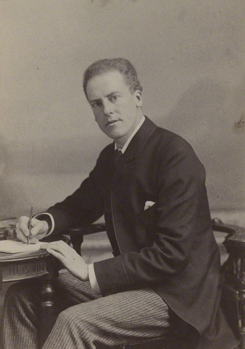
Figure: Karl Pearson (1857-1936), one of the founders of Mathematical Statistics.
Their movement did the most to put statistics to rights, to eradicate the ‘damned lies.’ It was known as ‘mathematical statistics’. Today I believe we should look to the emerging field of data science to provide the same role. Data science is an amalgam of statistics, data mining, computer systems, databases, computation, machine learning and artificial intelligence. Spread across these fields are the tools we need to realize data’s potential. For many businesses this might be thought of as the challenge of ‘converting bits into atoms.’ Bits: the data stored on computer, atoms: the physical manifestation of what we do; the transfer of goods, the delivery of service. From fungible to tangible. When solving a challenge through data there are a series of obstacles that need to be addressed.
Firstly, data awareness: what data you have and where its stored. Sometimes this includes changing your conception of what data is and how it can be obtained. From automated production lines to apps on employee smart phones. Often data is locked away: manual log books, confidential data, personal data. For increasing awareness an internal audit can help. The website data.gov.uk hosts data made available by the UK government. To create this website the government’s departments went through an audit of what data they each hold and what data they could make available. Similarly, within private buisnesses this type of audit could be useful for understanding their internal digital landscape: after all the key to any successful campaign is a good map.
Secondly, availability. How well are the data sources interconnected? How well curated are they? The curse of Disraeli was associated with unreliable data and unreliable statistics. The misrepresentations this leads to are worse than the absence of data as they give a false sense of confidence to decision making. Understanding how to avoid these pitfalls involves an improved sense of data and its value, one that needs to permeate the organization.
The final challenge is analysis, the accumulation of the necessary expertise to digest what the data tells us. Data requires intepretation, and interpretation requires experience. Analysis is providing a bottleneck due to a skill shortage, a skill shortage made more acute by the fact that, ideally, analysis should be carried out by individuals not only skilled in data science but also equipped with the domain knowledge to understand the implications in a given application, and to see opportunities for improvements in efficiency.
‘Mathematical Data Science’
As a term ‘big data’ promises much and delivers little, to get true value from data, it needs to be curated and evaluated. The three stages of awareness, availability and analysis provide a broad framework through which organizations should be assessing the potential in the data they hold. Hand waving about big data solutions will not do, it will only lead to self-deception. The castles we build on our data landscapes must be based on firm foundations, process and scientific analysis. If we do things right, those are the foundations that will be provided by the new field of data science.
Today the statement “There are three types of lies: lies, damned lies and ‘big data’” may be more apt. We are revisiting many of the mistakes made in interpreting data from the 19th century. Big data is laid down by happenstance, rather than actively collected with a particular question in mind. That means it needs to be treated with care when conclusions are being drawn. For data science to succede it needs the same form of rigour that Pearson and Fisher brought to statistics, a “mathematical data science” is needed.
You can also check my blog post on Lies, Damned Lies and Big Data.
Heider and Simmel (1944)
Figure: Fritz Heider and Marianne Simmel’s video of shapes from Heider and Simmel (1944).
Fritz Heider and Marianne Simmel’s experiments with animated shapes from 1944 (Heider and Simmel, 1944). Our interpretation of these objects as showing motives and even emotion is a combination of our desire for narrative, a need for understanding of each other, and our ability to empathise. At one level, these are crudely drawn objects, but in another key way, the animator has communicated a story through simple facets such as their relative motions, their sizes and their actions. We apply our psychological representations to these faceless shapes in an effort to interpret their actions.
See also a recent review paper on Human Cooperation by Henrich and Muthukrishna (2021).
Computer Conversations
Figure: Conversation relies on internal models of other individuals.
Figure: Misunderstanding of context and who we are talking to leads to arguments.
Similarly, we find it difficult to comprehend how computers are making decisions. Because they do so with more data than we can possibly imagine.
In many respects, this is not a problem, it’s a good thing. Computers and us are good at different things. But when we interact with a computer, when it acts in a different way to us, we need to remember why.
Just as the first step to getting along with other humans is understanding other humans, so it needs to be with getting along with our computers.
Embodiment factors explain why, at the same time, computers are so impressive in simulating our weather, but so poor at predicting our moods. Our complexity is greater than that of our weather, and each of us is tuned to read and respond to one another.
Their intelligence is different. It is based on very large quantities of data that we cannot absorb. Our computers don’t have a complex internal model of who we are. They don’t understand the human condition. They are not tuned to respond to us as we are to each other.
Embodiment factors encapsulate a profound thing about the nature of humans. Our locked in intelligence means that we are striving to communicate, so we put a lot of thought into what we’re communicating with. And if we’re communicating with something complex, we naturally anthropomorphize them.
We give our dogs, our cats and our cars human motivations. We do the same with our computers. We anthropomorphize them. We assume that they have the same objectives as us and the same constraints. They don’t.
This means, that when we worry about artificial intelligence, we worry about the wrong things. We fear computers that behave like more powerful versions of ourselves that will struggle to outcompete us.
In reality, the challenge is that our computers cannot be human enough. They cannot understand us with the depth we understand one another. They drop below our cognitive radar and operate outside our mental models.
The real danger is that computers don’t anthropomorphize. They’ll make decisions in isolation from us without our supervision, because they can’t communicate truly and deeply with us.
The Big Data Paradox
The big data paradox is the modern phenomenon of “as we collect more data, we understand less.” It is emerging in several domains, political polling, characterization of patients for trials data, monitoring twitter for political sentiment.
I like to think of the phenomenon as relating to the notion of “can’t see the wood for the trees.” Classical statistics, with randomized controlled trials, improved society’s understanding of data. It improved our ability to monitor the forest, to consider population health, voting patterns etc. It is critically dependent on active approaches to data collection that deal with confounders. This data collection can be very expensive.
In business today, it is still the gold standard, A/B tests are used to understand the effect of an intervention on revenue or customer capture or supply chain costs.

Figure: New beech leaves growing in the Gribskov Forest in the northern part of Sealand, Denmark. Photo from wikimedia commons by Malene Thyssen, http://commons.wikimedia.org/wiki/User:Malene.
The new phenomenon is happenstance data. Data that is not actively collected with a question in mind. As a result, it can mislead us. For example, if we assume the politics of active users of twitter is reflective of the wider population’s politics, then we may be misled.
However, this happenstance data often allows us to characterise a particular individual to a high degree of accuracy. Classical statistics was all about the forest, but big data can often become about the individual tree. As a result we are misled about the situation.
The phenomenon is more dangerous, because our perception is that we are characterizing the wider scenario with ever increasing accuracy. Whereas we are just becoming distracted by detail that may or may not be pertinent to the wider situation.
This is related to our limited bandwidth as humans, and the ease with which we are distracted by detail. The data-inattention-cognitive-bias.
Big Model Paradox
The big data paradox has a sister: the big model paradox. As we build more and more complex models, we start believing that we have a high-fidelity representation of reality. But the complexity of reality is way beyond our feeble imaginings. So we end up with a highly complex model, but one that falls well short in terms of reflecting reality. The complexity of the model means that it moves beyond our understanding.
Complexity in Action
As an exercise in understanding complexity, watch the following video. You will see the basketball being bounced around, and the players moving. Your job is to count the passes of those dressed in white and ignore those of the individuals dressed in black.
Figure: Daniel Simon’s famous illusion “monkey business.” Focus on the movement of the ball distracts the viewer from seeing other aspects of the image.
In a classic study Simons and Chabris (1999) ask subjects to count the number of passes of the basketball between players on the team wearing white shirts. Fifty percent of the time, these subjects don’t notice the gorilla moving across the scene.
The phenomenon of inattentional blindness is well known, e.g in their paper Simons and Charbris quote the Hungarian neurologist, Rezsö Bálint,
It is a well-known phenomenon that we do not notice anything happening in our surroundings while being absorbed in the inspection of something; focusing our attention on a certain object may happen to such an extent that we cannot perceive other objects placed in the peripheral parts of our visual field, although the light rays they emit arrive completely at the visual sphere of the cerebral cortex.
Rezsö Bálint 1907 (translated in Husain and Stein 1988, page 91)
When we combine the complexity of the world with our relatively low bandwidth for information, problems can arise. Our focus on what we perceive to be the most important problem can cause us to miss other (potentially vital) contextual information.
This phenomenon is known as selective attention or ‘inattentional blindness.’
Figure: For a longer talk on inattentional bias from Daniel Simons see this video.
Data Selective Attention Bias
We are going to see how inattention biases can play out in data analysis by going through a simple example. The analysis involves body mass index and activity information.
BMI Steps Data
The BMI Steps example is taken from Yanai and Lercher (2020). We are given a data set of body-mass index measurements against step counts. For convenience we have packaged the data so that it can be easily downloaded.
import podsdata = pods.datasets.bmi_steps()
X = data['X']
y = data['Y']It is good practice to give our variables interpretable names so that the analysis may be clearly understood by others. Here the steps count is the first dimension of the covariate, the bmi is the second dimension and the gender is stored in y with 1 for female and 0 for male.
steps = X[:, 0]
bmi = X[:, 1]
gender = y[:, 0]
We can check the mean steps and the mean of the BMI.
print('Steps mean is {mean}.'.format(mean=steps.mean()))print('BMI mean is {mean}.'.format(mean=bmi.mean()))BMI Steps Data Analysis
We can also separate out the means from the male and female populations. In python this can be done by setting male and female indices as follows.
male_ind = (gender==0)
female_ind = (gender==1)
And now we can extract the variables for the two populations.
male_steps = steps[male_ind]
male_bmi = bmi[male_ind]
And as before we compute the mean.
print('Male steps mean is {mean}.'.format(mean=male_steps.mean()))print('Male BMI mean is {mean}.'.format(mean=male_bmi.mean()))Similarly, we can get the same result for the female portion of the populaton.
female_steps = steps[female_ind]
female_bmi = bmi[female_ind]print('Female steps mean is {mean}.'.format(mean=female_steps.mean()))print('Female BMI mean is {mean}.'.format(mean=female_bmi.mean()))Interesting, the female BMI average is slightly higher than the male BMI average. The number of steps in the male group is higher than that in the female group. Perhaps the steps and the BMI are anti-correlated. The more steps, the lower the BMI.
Python provides a statistics package. We’ll import this in python so that we can try and understand the correlation between the steps and the BMI.
from scipy.stats import pearsonrcorr, _ = pearsonr(steps, bmi)
print("Pearson's overall correlation: {corr}".format(corr=corr))
male_corr, _ = pearsonr(male_steps, male_bmi)
print("Pearson's correlation for males: {corr}".format(corr=male_corr))
female_corr, _ = pearsonr(female_steps, female_bmi)
print("Pearson's correlation for females: {corr}".format(corr=female_corr))
A Hypothesis as a Liability
This analysis is from an article titled “A Hypothesis as a Liability” (Yanai and Lercher, 2020), they start their article with the following quite from Herman Hesse.
“ ‘When someone seeks,’ said Siddhartha, ‘then it easily happens that his eyes see only the thing that he seeks, and he is able to find nothing, to take in nothing. […] Seeking means: having a goal. But finding means: being free, being open, having no goal.’ ”
Hermann Hesse
Their idea is that having a hypothesis can constrain our thinking. However, in answer to their paper Felin et al. (2021) argue that some form of hypothesis is always necessary, suggesting that a hypothesis can be a liability
My view is captured in the introductory chapter to an edited volume on computational systems biology that I worked on with Mark Girolami, Magnus Rattray and Guido Sanguinetti.
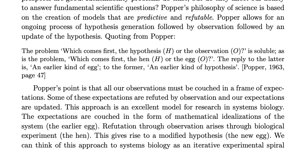
Figure: Quote from Lawrence (2010) highlighting the importance of interaction between data and hypothesis.
Popper nicely captures the interaction between hypothesis and data by relating it to the chicken and the egg. The important thing is that these two co-evolve.
Number Theatre
Unfortunately, we don’t always have time to wait for this process to converge to an answer we can all rely on before a decision is required.
Not only can we be misled by data before a decision is made, but sometimes we can be misled by data to justify the making of a decision. David Spiegelhalter refers to the phenomenon of “Number Theatre” in a conversation with Andrew Marr from May 2020 on the presentation of data.
Figure: Professor Sir David Spiegelhalter on Andrew Marr on 10th May 2020 speaking about some of the challengers around data, data presentation, and decision making in a pandemic. David mentions number theatre at 9 minutes 10 seconds.
Data Theatre
Data Theatre exploits data inattention bias to present a particular view on events that may misrepresents through selective presentation. Statisticians are one of the few groups that are trained with a sufficient degree of data skepticism. But it can also be combatted through ensuring there are domain experts present, and that they can speak freely.
Figure: The pheonomenon of number theatre or data theatre was described by David Spiegelhalter and is nicely sumamrized by Martin Robbins in this sub-stack article https://martinrobbins.substack.com/p/data-theatre-why-the-digital-dashboards.
The best book I have found for teaching the skeptical sense of data that underlies the statisticians craft is David Spiegelhalter’s Art of Statistics.
The Art of Statistics
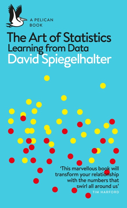
Figure: The Art of Statistics by David Spiegelhalter is an excellent read on the pitfalls of data interpretation.
David’s (Spiegelhalter, 2019) book brings important examples from statistics to life in an intelligent and entertaining way. It is highly readable and gives an opportunity to fast-track towards the important skill of data-skepticism that is the mark of a professional statistician.
Conclusion
See the Gorilla don’t be the Gorilla.

Figure: A famous quote from Mike Tyson before his fight with Evander Holyfield: “Everyone has a plan until they get punched in the mouth.” Don’t let the gorilla punch you in the mouth. See the gorilla, but don’t be the gorilla. Photo credit: https://www.catersnews.com/stories/animals/go-ape-unlucky-photographer-gets-punched-by-lairy-gorilla-drunk-from-eating-bamboo-shoots/
Thanks!
For more information on these subjects and more you might want to check the following resources.
- twitter: @lawrennd
- podcast: The Talking Machines
- newspaper: Guardian Profile Page
- blog: http://inverseprobability.com