AI4ER Lecture: Projects
Abstract
In this session we look at some projects from data science africa and review challenges around ethical artificial intelligence from a perspective of data governance. We’ll give some background to how these challenges have emerged and then consider some solutions including the mechanism of data trusts and some pointers to work around data sharing in Africa for the Covid19 pandemic.
Lies and Damned Lies
There are three types of lies: lies, damned lies and statistics
Benjamin Disraeli 1804-1881
Benjamin Disraeli said1 that there three types of lies: lies, damned lies and statistics. Disraeli died in 1881, 30 years before the first academic department of applied statistics was founded at UCL. If Disraeli were alive today, it is likely that he’d rephrase his quote:
There are three types of lies, lies damned lies and big data.
Why? Because the challenges of understanding and interpreting big data today are similar to those that Disraeli faced in governing an empire through statistics in the latter part of the 19th century.
The quote lies, damned lies and statistics was credited to Benjamin Disraeli by Mark Twain in his autobiography. It characterizes the idea that statistic can be made to prove anything. But Disraeli died in 1881 and Mark Twain died in 1910. The important breakthrough in overcoming our tendency to overinterpet data came with the formalization of the field through the development of mathematical statistics.
Data has an elusive quality, it promises so much but can deliver little, it can mislead and misrepresent. To harness it, it must be tamed. In Disraeli’s time during the second half of the 19th century, numbers and data were being accumulated, the social sciences were being developed. There was a large scale collection of data for the purposes of government.
The modern ‘big data era’ is on the verge of delivering the same sense of frustration that Disraeli experienced, the early promise of big data as a panacea is evolving to demands for delivery. For me, personally, peak-hype coincided with an email I received inviting collaboration on a project to deploy “Big Data and Internet of Things in an Industry 4.0 environment.” Further questioning revealed that the actual project was optimization of the efficiency of a manufacturing production line, a far more tangible and realizable goal.
The antidote to this verbage is found in increasing awareness. When dealing with data the first trap to avoid is the games of buzzword bingo that we are wont to play. The first goal is to quantify what challenges can be addressed and what techniques are required. Behind the hype fundamentals are changing. The phenomenon is about the increasing access we have to data. The manner in which customers information is recorded and processes are codified and digitized with little overhead. Internet of things is about the increasing number of cheap sensors that can be easily interconnected through our modern network structures. But businesses are about making money, and these phenomena need to be recast in those terms before their value can be realized.
Mathematical Statistics
Karl Pearson (1857-1936), Ronald Fisher (1890-1962) and others considered the question of what conclusions can truly be drawn from data. Their mathematical studies act as a restraint on our tendency to over-interpret and see patterns where there are none. They introduced concepts such as randomized control trials that form a mainstay of the our decision making today, from government, to clinicians to large scale A/B testing that determines the nature of the web interfaces we interact with on social media and shopping.


Figure: Karl Pearson (1857-1936), one of the founders of Mathematical Statistics.
Their movement did the most to put statistics to rights, to eradicate the ‘damned lies.’ It was known as ‘mathematical statistics’. Today I believe we should look to the emerging field of data science to provide the same role. Data science is an amalgam of statistics, data mining, computer systems, databases, computation, machine learning and artificial intelligence. Spread across these fields are the tools we need to realize data’s potential. For many businesses this might be thought of as the challenge of ‘converting bits into atoms.’ Bits: the data stored on computer, atoms: the physical manifestation of what we do; the transfer of goods, the delivery of service. From fungible to tangible. When solving a challenge through data there are a series of obstacles that need to be addressed.
Firstly, data awareness: what data you have and where its stored. Sometimes this includes changing your conception of what data is and how it can be obtained. From automated production lines to apps on employee smart phones. Often data is locked away: manual log books, confidential data, personal data. For increasing awareness an internal audit can help. The website data.gov.uk hosts data made available by the UK government. To create this website the government’s departments went through an audit of what data they each hold and what data they could make available. Similarly, within private buisnesses this type of audit could be useful for understanding their internal digital landscape: after all the key to any successful campaign is a good map.
Secondly, availability. How well are the data sources interconnected? How well curated are they? The curse of Disraeli was associated with unreliable data and unreliable statistics. The misrepresentations this leads to are worse than the absence of data as they give a false sense of confidence to decision making. Understanding how to avoid these pitfalls involves an improved sense of data and its value, one that needs to permeate the organization.
The final challenge is analysis, the accumulation of the necessary expertise to digest what the data tells us. Data requires intepretation, and interpretation requires experience. Analysis is providing a bottleneck due to a skill shortage, a skill shortage made more acute by the fact that, ideally, analysis should be carried out by individuals not only skilled in data science but also equipped with the domain knowledge to understand the implications in a given application, and to see opportunities for improvements in efficiency.
‘Mathematical Data Science’
As a term ‘big data’ promises much and delivers little, to get true value from data, it needs to be curated and evaluated. The three stages of awareness, availability and analysis provide a broad framework through which organizations should be assessing the potential in the data they hold. Hand waving about big data solutions will not do, it will only lead to self-deception. The castles we build on our data landscapes must be based on firm foundations, process and scientific analysis. If we do things right, those are the foundations that will be provided by the new field of data science.
Today the statement “There are three types of lies: lies, damned lies and ‘big data’” may be more apt. We are revisiting many of the mistakes made in interpreting data from the 19th century. Big data is laid down by happenstance, rather than actively collected with a particular question in mind. That means it needs to be treated with care when conclusions are being drawn. For data science to succede it needs the same form of rigour that Pearson and Fisher brought to statistics, a “mathematical data science” is needed.
You can also check my blog post on Lies, Damned Lies and Big Data.
Embodiment Factors
| bits/min | billions | 2,000 |
|
billion calculations/s |
~100 | a billion |
| embodiment | 20 minutes | 5 billion years |
Figure: Embodiment factors are the ratio between our ability to compute and our ability to communicate. Relative to the machine we are also locked in. In the table we represent embodiment as the length of time it would take to communicate one second’s worth of computation. For computers it is a matter of minutes, but for a human, it is a matter of thousands of millions of years. See also “Living Together: Mind and Machine Intelligence” Lawrence (2017)
There is a fundamental limit placed on our intelligence based on our ability to communicate. Claude Shannon founded the field of information theory. The clever part of this theory is it allows us to separate our measurement of information from what the information pertains to.2
Shannon measured information in bits. One bit of information is the amount of information I pass to you when I give you the result of a coin toss. Shannon was also interested in the amount of information in the English language. He estimated that on average a word in the English language contains 12 bits of information.
Given typical speaking rates, that gives us an estimate of our ability to communicate of around 100 bits per second (Reed and Durlach, 1998). Computers on the other hand can communicate much more rapidly. Current wired network speeds are around a billion bits per second, ten million times faster.
When it comes to compute though, our best estimates indicate our computers are slower. A typical modern computer can process make around 100 billion floating point operations per second, each floating point operation involves a 64 bit number. So the computer is processing around 6,400 billion bits per second.
It’s difficult to get similar estimates for humans, but by some estimates the amount of compute we would require to simulate a human brain is equivalent to that in the UK’s fastest computer (Ananthanarayanan et al., 2009), the MET office machine in Exeter, which in 2018 ranks as the 11th fastest computer in the world. That machine simulates the world’s weather each morning, and then simulates the world’s climate in the afternoon. It is a 16 petaflop machine, processing around 1,000 trillion bits per second.
Bandwidth Constrained Conversations
Figure: Conversation relies on internal models of other individuals.
Figure: Misunderstanding of context and who we are talking to leads to arguments.
Embodiment factors imply that, in our communication between humans, what is not said is, perhaps, more important than what is said. To communicate with each other we need to have a model of who each of us are.
To aid this, in society, we are required to perform roles. Whether as a parent, a teacher, an employee or a boss. Each of these roles requires that we conform to certain standards of behaviour to facilitate communication between ourselves.
Control of self is vitally important to these communications.
The high availability of data available to humans undermines human-to-human communication channels by providing new routes to undermining our control of self.
The consequences between this mismatch of power and delivery are to be seen all around us. Because, just as driving an F1 car with bicycle wheels would be a fine art, so is the process of communication between humans.
If I have a thought and I wish to communicate it, I first of all need to have a model of what you think. I should think before I speak. When I speak, you may react. You have a model of who I am and what I was trying to say, and why I chose to say what I said. Now we begin this dance, where we are each trying to better understand each other and what we are saying. When it works, it is beautiful, but when misdeployed, just like a badly driven F1 car, there is a horrible crash, an argument.
Computer Conversations
Figure: Conversation relies on internal models of other individuals.
Figure: Misunderstanding of context and who we are talking to leads to arguments.
Similarly, we find it difficult to comprehend how computers are making decisions. Because they do so with more data than we can possibly imagine.
In many respects, this is not a problem, it’s a good thing. Computers and us are good at different things. But when we interact with a computer, when it acts in a different way to us, we need to remember why.
Just as the first step to getting along with other humans is understanding other humans, so it needs to be with getting along with our computers.
Embodiment factors explain why, at the same time, computers are so impressive in simulating our weather, but so poor at predicting our moods. Our complexity is greater than that of our weather, and each of us is tuned to read and respond to one another.
Their intelligence is different. It is based on very large quantities of data that we cannot absorb. Our computers don’t have a complex internal model of who we are. They don’t understand the human condition. They are not tuned to respond to us as we are to each other.
Embodiment factors encapsulate a profound thing about the nature of humans. Our locked in intelligence means that we are striving to communicate, so we put a lot of thought into what we’re communicating with. And if we’re communicating with something complex, we naturally anthropomorphize them.
We give our dogs, our cats and our cars human motivations. We do the same with our computers. We anthropomorphize them. We assume that they have the same objectives as us and the same constraints. They don’t.
This means, that when we worry about artificial intelligence, we worry about the wrong things. We fear computers that behave like more powerful versions of ourselves that will struggle to outcompete us.
In reality, the challenge is that our computers cannot be human enough. They cannot understand us with the depth we understand one another. They drop below our cognitive radar and operate outside our mental models.
The real danger is that computers don’t anthropomorphize. They’ll make decisions in isolation from us without our supervision, because they can’t communicate truly and deeply with us.
Evolved Relationship with Information
The high bandwidth of computers has resulted in a close relationship between the computer and data. Large amounts of information can flow between the two. The degree to which the computer is mediating our relationship with data means that we should consider it an intermediary.
Originaly our low bandwith relationship with data was affected by two characteristics. Firstly, our tendency to over-interpret driven by our need to extract as much knowledge from our low bandwidth information channel as possible. Secondly, by our improved understanding of the domain of mathematical statistics and how our cognitive biases can mislead us.
With this new set up there is a potential for assimilating far more information via the computer, but the computer can present this to us in various ways. If it’s motives are not aligned with ours then it can misrepresent the information. This needn’t be nefarious it can be simply as a result of the computer pursuing a different objective from us. For example, if the computer is aiming to maximize our interaction time that may be a different objective from ours which may be to summarize information in a representative manner in the shortest possible length of time.
For example, for me, it was a common experience to pick up my telephone with the intention of checking when my next appointment was, but to soon find myself distracted by another application on the phone, and end up reading something on the internet. By the time I’d finished reading, I would often have forgotten the reason I picked up my phone in the first place.
There are great benefits to be had from the huge amount of information we can unlock from this evolved relationship between us and data. In biology, large scale data sharing has been driven by a revolution in genomic, transcriptomic and epigenomic measurement. The improved inferences that can be drawn through summarizing data by computer have fundamentally changed the nature of biological science, now this phenomenon is also infuencing us in our daily lives as data measured by happenstance is increasingly used to characterize us.
Better mediation of this flow actually requires a better understanding of human-computer interaction. This in turn involves understanding our own intelligence better, what its cognitive biases are and how these might mislead us.
For further thoughts see Guardian article on marketing in the internet era from 2015.
You can also check my blog post on System Zero. also from 2015.
New Flow of Information
Classically the field of statistics focussed on mediating the relationship between the machine and the human. Our limited bandwidth of communication means we tend to over-interpret the limited information that we are given, in the extreme we assign motives and desires to inanimate objects (a process known as anthropomorphizing). Much of mathematical statistics was developed to help temper this tendency and understand when we are valid in drawing conclusions from data.
Figure: The trinity of human, data and computer, and highlights the modern phenomenon. The communication channel between computer and data now has an extremely high bandwidth. The channel between human and computer and the channel between data and human is narrow. New direction of information flow, information is reaching us mediated by the computer. The focus on classical statistics reflected the importance of the direct communication between human and data. The modern challenges of data science emerge when that relationship is being mediated by the machine.
Data science brings new challenges. In particular, there is a very large bandwidth connection between the machine and data. This means that our relationship with data is now commonly being mediated by the machine. Whether this is in the acquisition of new data, which now happens by happenstance rather than with purpose, or the interpretation of that data where we are increasingly relying on machines to summarise what the data contains. This is leading to the emerging field of data science, which must not only deal with the same challenges that mathematical statistics faced in tempering our tendency to over interpret data, but must also deal with the possibility that the machine has either inadvertently or malisciously misrepresented the underlying data.
The Gartner Hype Cycle
Figure: The Gartner Hype Cycle places technologies on a graph that relates to the expectations we have of a technology against its actual influence. Early hope for a new techology is often displaced by disillusionment due to the time it takes for a technology to be usefully deployed.
The Gartner Hype Cycle tries to assess where an idea is in terms of maturity and adoption. It splits the evolution of technology into a technological trigger, a peak of expectations followed by a trough of disillusionment and a final ascension into a useful technology. It looks rather like a classical control response to a final set point.
Cycle for ML Terms
Google Trends
%pip install pytrendsFigure: Google trends for ‘artificial intelligence,’ ‘big data,’ ‘data mining,’ ‘deep learning,’ ‘machine learning’ as different technological terms gives us insight into their popularity over time.
Google trends gives us insight into the interest for different terms over time.
Examining Google treds for ‘artificial intelligence,’ ‘big data,’ ‘data mining,’ ‘deep learning’ and ‘machine learning’ we can see that ‘artificial intelligence’ may be entering a plateau of productivity, ‘big data’ is entering the trough of disillusionment, and ‘data mining’ seems to be deeply within the trough. On the other hand, ‘deep learning’ and ‘machine learning’ appear to be ascending to the peak of inflated expectations having experienced a technology trigger.
For deep learning that technology trigger was the ImageNet result of 2012 (Krizhevsky et al., n.d.). This step change in performance on object detection in images was achieved through convolutional neural networks, popularly known as ‘deep learning.’
Challenges
The field of data science is rapidly evolving. Different practitioners from different domains have their own perspectives. We identify three broad challenges that are emerging. Challenges which have not been addressed in the traditional sub-domains of data science. The challenges have social implications but require technological advance for their solutions.
- Paradoxes of the Data Society
- Quantifying the Value of Data
- Privacy, loss of control, marginalization
You can also check this blog post on Three Data Science Challenges..
Privacy, Loss of Control and Marginalization
Society is becoming harder to monitor, but the individual is becoming easier to monitor. Social media monitoring for ‘hate speech’ can easily be turned to monitoring of political dissent. Marketing becomes more sinister when the target of the marketing is so well understood and the digital environment of the target is so well controlled.
There is potential for both explicit and implicit discrimination on the basis of race, religion, sexuality or health status. All of these are prohibited under European law, but can pass unawares or be implicit.
The GDPR is the General Data Protection Regulation, but a better name for it would simpl by Good Data Practice Rules. It covers how to deal with discrimination which has a consequential effect on the individual. For example, entrance to University, access to loans or insurance. But the new phenomenon is dealing with a series of inconsequential decisions that taken together have a consequential effect.

Figure: A woman tends her house in a village in Uganda.
Statistics as a community is also focussed on the single consequential effect of an analysis (efficacy of drugs, or distribution of Mosquito nets). Associated with happenstance data is happenstance decision making.
These algorithms behind these decisions are developed in a particular context. The so-called Silicon Valley bubble. But they are deployed across the world. To address this, a key challenge is capacity building in contexts which are remote from the Western norm.
Data Science Africa
Figure: Data Science Africa http://datascienceafrica.org is a ground up initiative for capacity building around data science, machine learning and artificial intelligence on the African continent.
Figure: Data Science Africa meetings held up to October 2021.
Data Science Africa is a bottom up initiative for capacity building in data science, machine learning and artificial intelligence on the African continent.
As of October 2021 there have been five workshops and five schools, located in Nyeri, Kenya (twice); Kampala, Uganda; Arusha, Tanzania; Abuja, Nigeria; Addis Ababa, Ethiopia; Accra, Ghana; Kampala, Uganda and Kimberley, South Africa.
The main notion is end-to-end data science. For example, going from data collection in the farmer’s field to decision making in the Ministry of Agriculture. Or going from malaria disease counts in health centers to medicine distribution.
The philosophy is laid out in (Lawrence, 2015). The key idea is that the modern information infrastructure presents new solutions to old problems. Modes of development change because less capital investment is required to take advantage of this infrastructure. The philosophy is that local capacity building is the right way to leverage these challenges in addressing data science problems in the African context.
Data Science Africa is now a non-govermental organization registered in Kenya. The organising board of the meeting is entirely made up of scientists and academics based on the African continent.
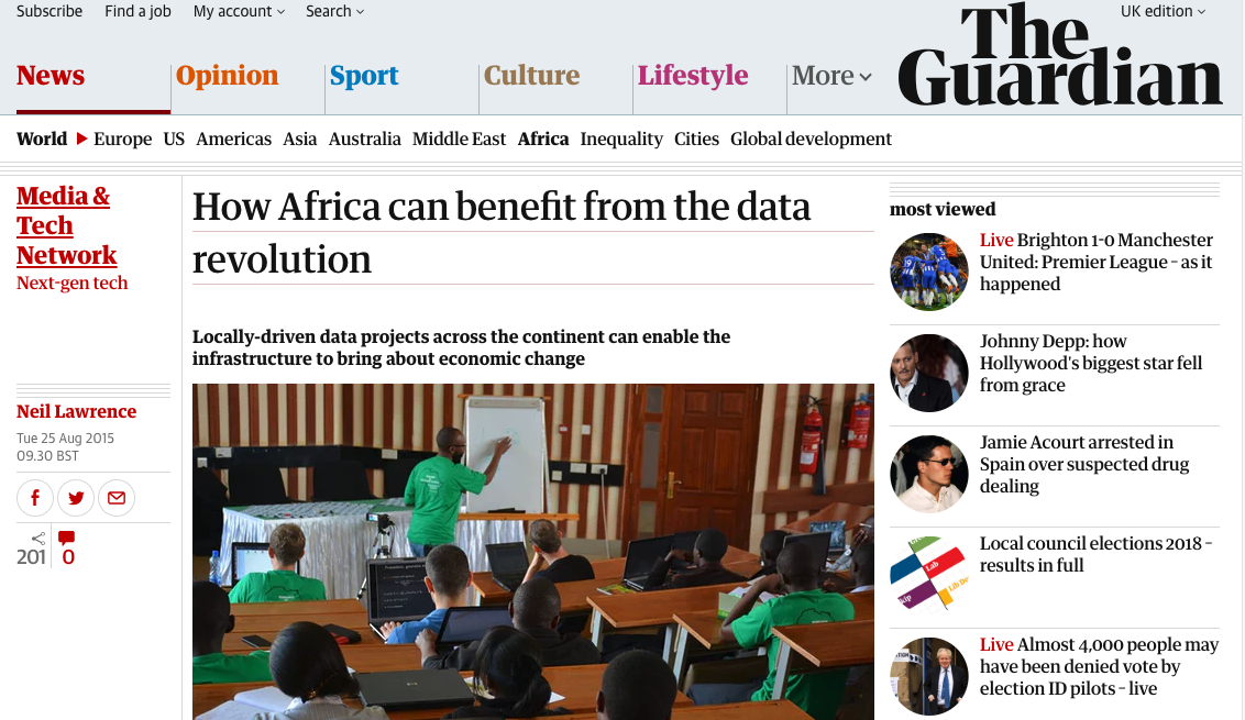
Figure: The lack of existing physical infrastructure on the African continent makes it a particularly interesting environment for deploying solutions based on the information infrastructure. The idea is explored more in this Guardian op-ed on Guardian article on How African can benefit from the data revolution.
Guardian article on Data Science Africa
Example: Prediction of Malaria Incidence in Uganda
As an example of using Gaussian process models within the full pipeline from data to decsion, we’ll consider the prediction of Malaria incidence in Uganda. For the purposes of this study malaria reports come in two forms, HMIS reports from health centres and Sentinel data, which is curated by the WHO. There are limited sentinel sites and many HMIS sites.
The work is from Ricardo Andrade Pacheco’s PhD thesis, completed in collaboration with John Quinn and Martin Mubangizi (Andrade-Pacheco et al., 2014; Mubangizi et al., 2014). John and Martin were initally from the AI-DEV group from the University of Makerere in Kampala and more latterly they were based at UN Global Pulse in Kampala. You can see the work summarized on the UN Global Pulse disease outbreaks project site here.
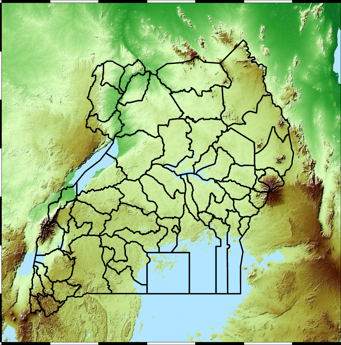
Malaria data is spatial data. Uganda is split into districts, and health reports can be found for each district. This suggests that models such as conditional random fields could be used for spatial modelling, but there are two complexities with this. First of all, occasionally districts split into two. Secondly, sentinel sites are a specific location within a district, such as Nagongera which is a sentinel site based in the Tororo district.
The common standard for collecting health data on the African continent is from the Health management information systems (HMIS). However, this data suffers from missing values (Gething et al., 2006) and diagnosis of diseases like typhoid and malaria may be confounded.
Figure: The Tororo district, where the sentinel site, Nagongera, is located.
World Health Organization Sentinel Surveillance systems are set up “when high-quality data are needed about a particular disease that cannot be obtained through a passive system.” Several sentinel sites give accurate assessment of malaria disease levels in Uganda, including a site in Nagongera.
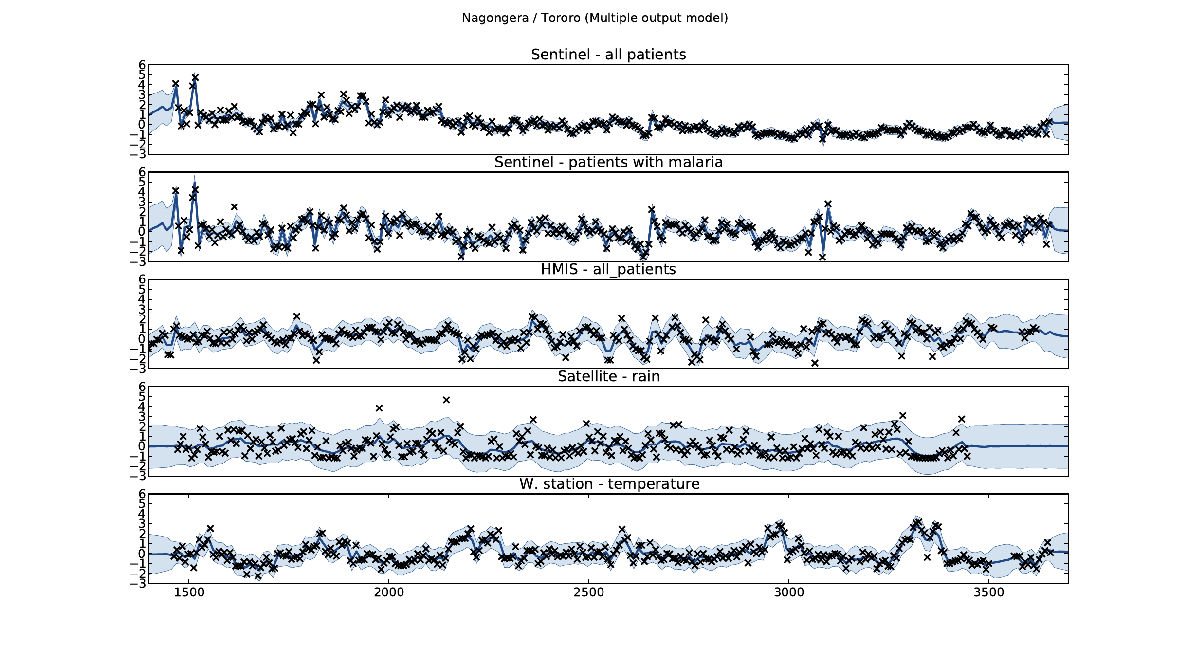
Figure: Sentinel and HMIS data along with rainfall and temperature for the Nagongera sentinel station in the Tororo district.
In collaboration with the AI Research Group at Makerere we chose to investigate whether Gaussian process models could be used to assimilate information from these two different sources of disease informaton. Further, we were interested in whether local information on rainfall and temperature could be used to improve malaria estimates.
The aim of the project was to use WHO Sentinel sites, alongside rainfall and temperature, to improve predictions from HMIS data of levels of malaria.
Figure: The Mubende District.
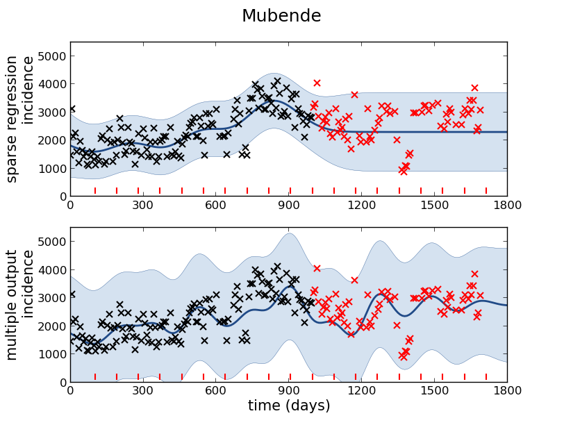
Figure: Prediction of malaria incidence in Mubende.
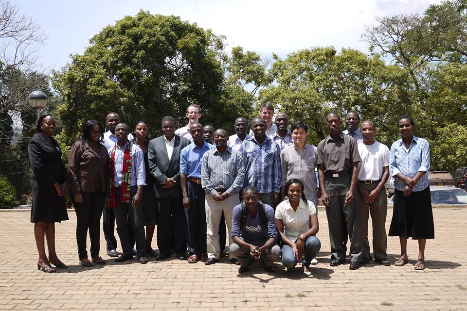
Figure: The project arose out of the Gaussian process summer school held at Makerere in Kampala in 2013. The school led, in turn, to the Data Science Africa initiative.
Early Warning Systems
Figure: The Kabarole district in Uganda.
Figure: Estimate of the current disease situation in the Kabarole district over time. Estimate is constructed with a Gaussian process with an additive covariance funciton.
Health monitoring system for the Kabarole district. Here we have fitted the reports with a Gaussian process with an additive covariance function. It has two components, one is a long time scale component (in red above) the other is a short time scale component (in blue).
Monitoring proceeds by considering two aspects of the curve. Is the blue line (the short term report signal) above the red (which represents the long term trend? If so we have higher than expected reports. If this is the case and the gradient is still positive (i.e. reports are going up) we encode this with a red color. If it is the case and the gradient of the blue line is negative (i.e. reports are going down) we encode this with an amber color. Conversely, if the blue line is below the red and decreasing, we color green. On the other hand if it is below red but increasing, we color yellow.
This gives us an early warning system for disease. Red is a bad situation getting worse, amber is bad, but improving. Green is good and getting better and yellow good but degrading.
Finally, there is a gray region which represents when the scale of the effect is small.
Figure: The map of Ugandan districts with an overview of the Malaria situation in each district.
These colors can now be observed directly on a spatial map of the districts to give an immediate impression of the current status of the disease across the country.
Crop Monitoring
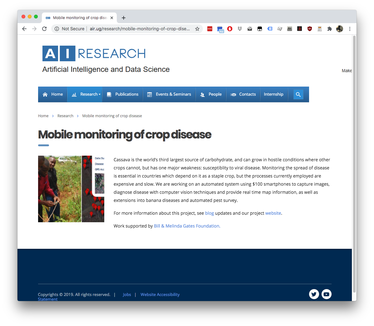
Figure: Mobile Monitoring of Crop Disease
Ernest’s Talk
You can see more details on Ernest’s work in this talk from the 2021 DNN lectures.
Figure: Lecture from Ernest Mwebaze on Deep Learning for Developmental Challenges
Biosurveillance
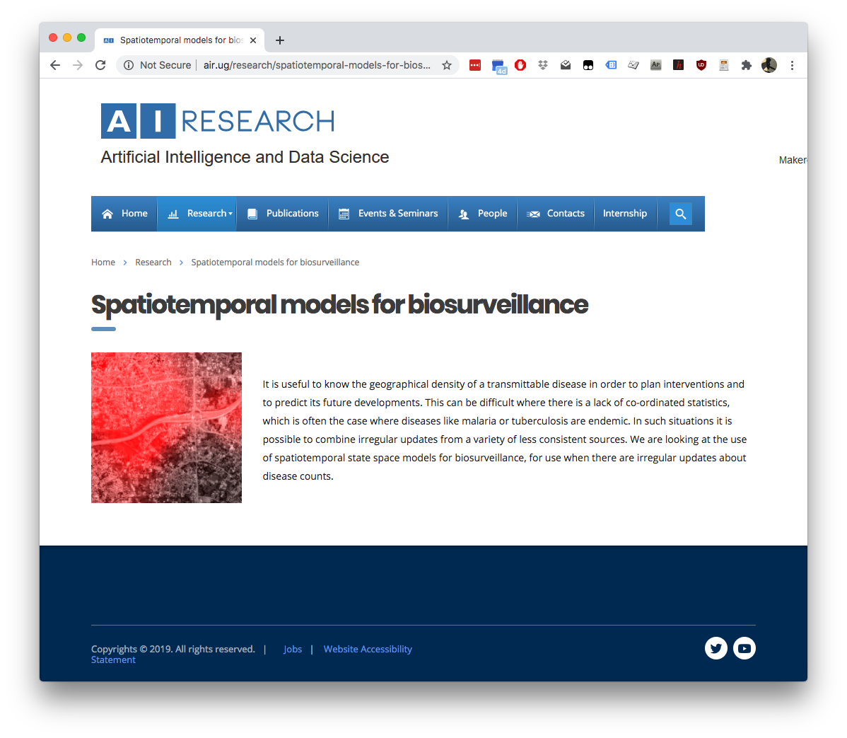
Figure: Spatiotemporal Models for Biosurveillance
Community Radio

Figure: Ugandan Community Radio Project
Kudu Project

Figure: Kudu Project
Safe Boda
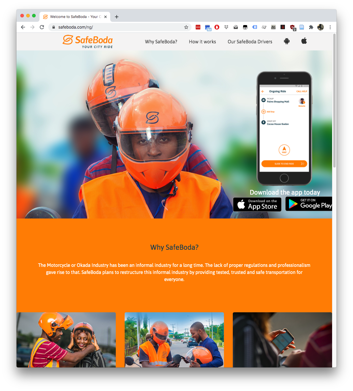
Figure: Safe Boda
Feudal Era Data Ecosystem
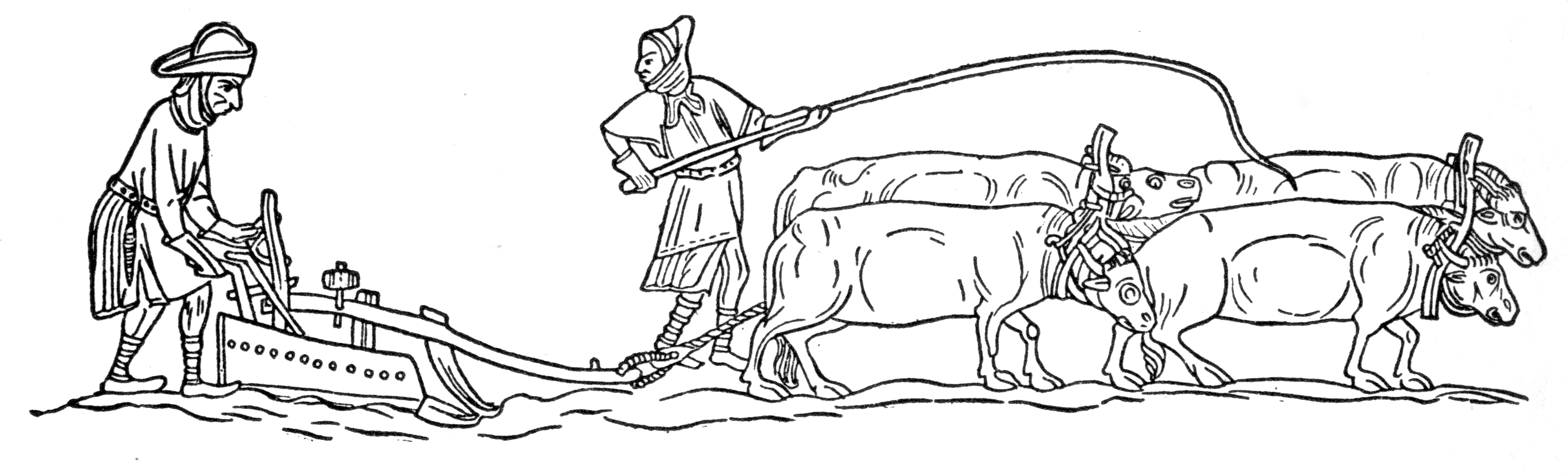
Figure: Feudal systems consist of serfs and vassals who are under the protection of a Lord. The Lord has a duty of care over the vassals, but due to power asymmetries that duty of care can be difficult to monitor and enforce. This is similar to the way our information is managed. Data controllers have a duty of care towards their data subjects, but there is also a power asymmetry between controller and subject.
Our current information infrastructure bears a close relation with feudal systems of government. In the feudal system a lord had a duty of care over his serfs and vassals, a duty to protect subjects. But in practice there was a power-asymetry. In feudal days protection was against Viking raiders, today, it is against information raiders. However, when there is an information leak, when there is some failure in protections, it is already too late.
Alternatively, our data is publicly shared, as in an information commons. Akin to common land of the medieval village. But just as commons were subject to overgrazing and poor management, so it is that much of our data cannot be managed in this way. In particularly personal, sensitive data.
I explored this idea further in this Guardian article on 2015/nov/16/information-barons-threaten-autonomy-privacy-online.
African Data Sharing Covid-19
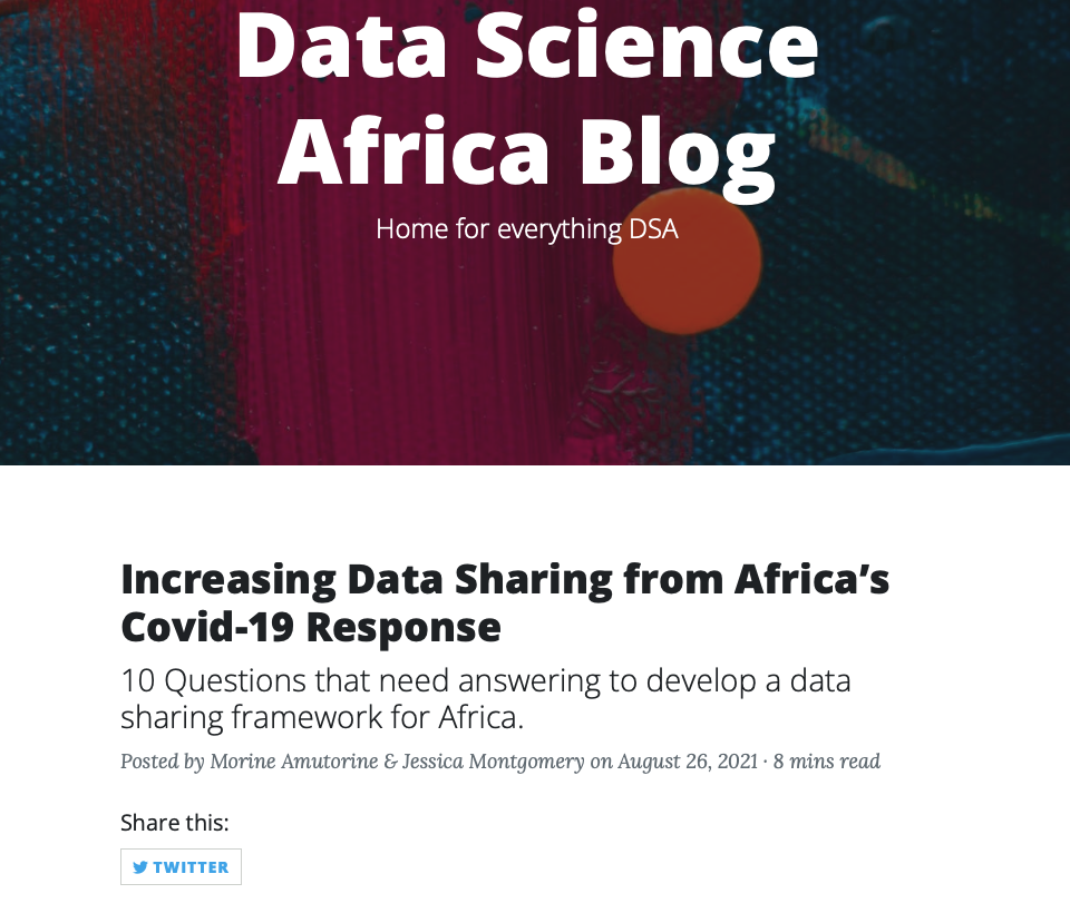
Figure: Blog post, https://www.datascienceafrica.org/dsablog/, by Morine Amutorine and Jessica Montgomery summarising some of the issues around data sharing in the Covid-19 response
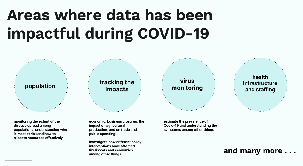
Figure: Areas where data has been impactful summarised from Morine Amutorine’s survey work on data sharing in Africa during the Covid19 response.
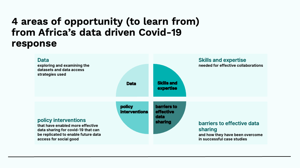
Figure: Four areas of opportunity to learn from identified by Morine Amutorine in her survey work on Africa’s data driven Covid-19 response.
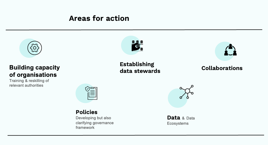
Figure: Areas for action arising from Morine Amutorine’s survey work on Africa’s data driven Covid-19 response.
Morine’s Areas for Action
Building capacity of organisations in the public and private sector to reuse and act on data through investments in training, education, and reskilling of relevant authorities;
Establishing data stewards in organisations who can coordinate and collaborate with counterparts on using data in the public’s interest and acting on it.
Technical skills and expertise-researchers (eg data scientists) to develop and deploy useful, privacy-preserving technologies.
Developing but also clarifying governance framework to enable the trusted, transparent, and accountable reuse of privately held data in the public interest under a clear regulatory framework
Data Collaboratives are a new form of collaboration, beyond the public-private partnership model, in which participants from different sectors — in particular companies - exchange their data to create public value.
References
Thanks!
For more information on these subjects and more you might want to check the following resources.
- twitter: @lawrennd
- podcast: The Talking Machines
- newspaper: Guardian Profile Page
- blog: http://inverseprobability.com
the challenge of understanding what information pertains to is known as knowledge representation.↩︎