Links

Abstract

Machine learning methods and software are becoming widely deployed. But how are we sharing expertise about bottlenecks and pain points in deploying solutions? In terms of the practice of data science, we seem to be at a similar point today as software engineering was in the early 1980s. Best practice is not widely understood or deployed. In this talk we will focus on two particular components of data science solutions: the preparation of data snd the deployment of machine learning systems.

What is Machine Learning?

What is machine learning? At its most basic level machine learning is a combination of

\[\text{data} + \text{model} \stackrel{\text{compute}}{\rightarrow} \text{prediction}\]

where data is our observations. They can be actively or passively acquired (meta-data). The model contains our assumptions, based on previous experience. That experience can be other data, it can come from transfer learning, or it can merely be our beliefs about the regularities of the universe. In humans our models include our inductive biases. The prediction is an action to be taken or a categorization or a quality score. The reason that machine learning has become a mainstay of artificial intelligence is the importance of predictions in artificial intelligence. The data and the model are combined through computation.

In practice we normally perform machine learning using two functions. To combine data with a model we typically make use of:

a prediction function a function which is used to make the predictions. It includes our beliefs about the regularities of the universe, our assumptions about how the world works, e.g., smoothness, spatial similarities, temporal similarities.

an objective function a function which defines the cost of misprediction. Typically, it includes knowledge about the world’s generating processes (probabilistic objectives) or the costs we pay for mispredictions (empirical risk minimization).

The combination of data and model through the prediction function and the objective function leads to a learning algorithm. The class of prediction functions and objective functions we can make use of is restricted by the algorithms they lead to. If the prediction function or the objective function are too complex, then it can be difficult to find an appropriate learning algorithm. Much of the academic field of machine learning is the quest for new learning algorithms that allow us to bring different types of models and data together.

A useful reference for state of the art in machine learning is the UK Royal Society Report, Machine Learning: Power and Promise of Computers that Learn by Example.

You can also check my post blog post on What is Machine Learning?.

Artificial Intelligence and Data Science

Machine learning technologies have been the driver of two related, but distinct disciplines. The first is data science. Data science is an emerging field that arises from the fact that we now collect so much data by happenstance, rather than by experimental design. Classical statistics is the science of drawing conclusions from data, and to do so statistical experiments are carefully designed. In the modern era we collect so much data that there’s a desire to draw inferences directly from the data.

As well as machine learning, the field of data science draws from statistics, cloud computing, data storage (e.g. streaming data), visualization and data mining.

In contrast, artificial intelligence technologies typically focus on emulating some form of human behaviour, such as understanding an image, or some speech, or translating text from one form to another. The recent advances in artifcial intelligence have come from machine learning providing the automation. But in contrast to data science, in artifcial intelligence the data is normally collected with the specific task in mind. In this sense it has strong relations to classical statistics.

Classically artificial intelligence worried more about logic and planning and focussed less on data driven decision making. Modern machine learning owes more to the field of Cybernetics (Wiener, 1948) than artificial intelligence. Related fields include robotics, speech recognition, language understanding and computer vision.

There are strong overlaps between the fields, the wide availability of data by happenstance makes it easier to collect data for designing AI systems. These relations are coming through wide availability of sensing technologies that are interconnected by celluar networks, WiFi and the internet. This phenomenon is sometimes known as the Internet of Things, but this feels like a dangerous misnomer. We must never forget that we are interconnecting people, not things.

Embodiment Factors

bits/min	billions	2,000
billion calculations/s	~100	a billion
embodiment	20 minutes	5 billion years

Figure: Embodiment factors are the ratio between our ability to compute and our ability to communicate. Relative to the machine we are also locked in. In the table we represent embodiment as the length of time it would take to communicate one second’s worth of computation. For computers it is a matter of minutes, but for a human, it is a matter of thousands of millions of years. See also “Living Together: Mind and Machine Intelligence” Lawrence (2017a)

There is a fundamental limit placed on our intelligence based on our ability to communicate. Claude Shannon founded the field of information theory. The clever part of this theory is it allows us to separate our measurement of information from what the information pertains to.¹

Shannon measured information in bits. One bit of information is the amount of information I pass to you when I give you the result of a coin toss. Shannon was also interested in the amount of information in the English language. He estimated that on average a word in the English language contains 12 bits of information.

Given typical speaking rates, that gives us an estimate of our ability to communicate of around 100 bits per second (Reed and Durlach, 1998). Computers on the other hand can communicate much more rapidly. Current wired network speeds are around a billion bits per second, ten million times faster.

When it comes to compute though, our best estimates indicate our computers are slower. A typical modern computer can process make around 100 billion floating point operations per second, each floating point operation involves a 64 bit number. So the computer is processing around 6,400 billion bits per second.

It’s difficult to get similar estimates for humans, but by some estimates the amount of compute we would require to simulate a human brain is equivalent to that in the UK’s fastest computer (Ananthanarayanan et al., 2009), the MET office machine in Exeter, which in 2018 ranks as the 11th fastest computer in the world. That machine simulates the world’s weather each morning, and then simulates the world’s climate in the afternoon. It is a 16 petaflop machine, processing around 1,000 trillion bits per second.

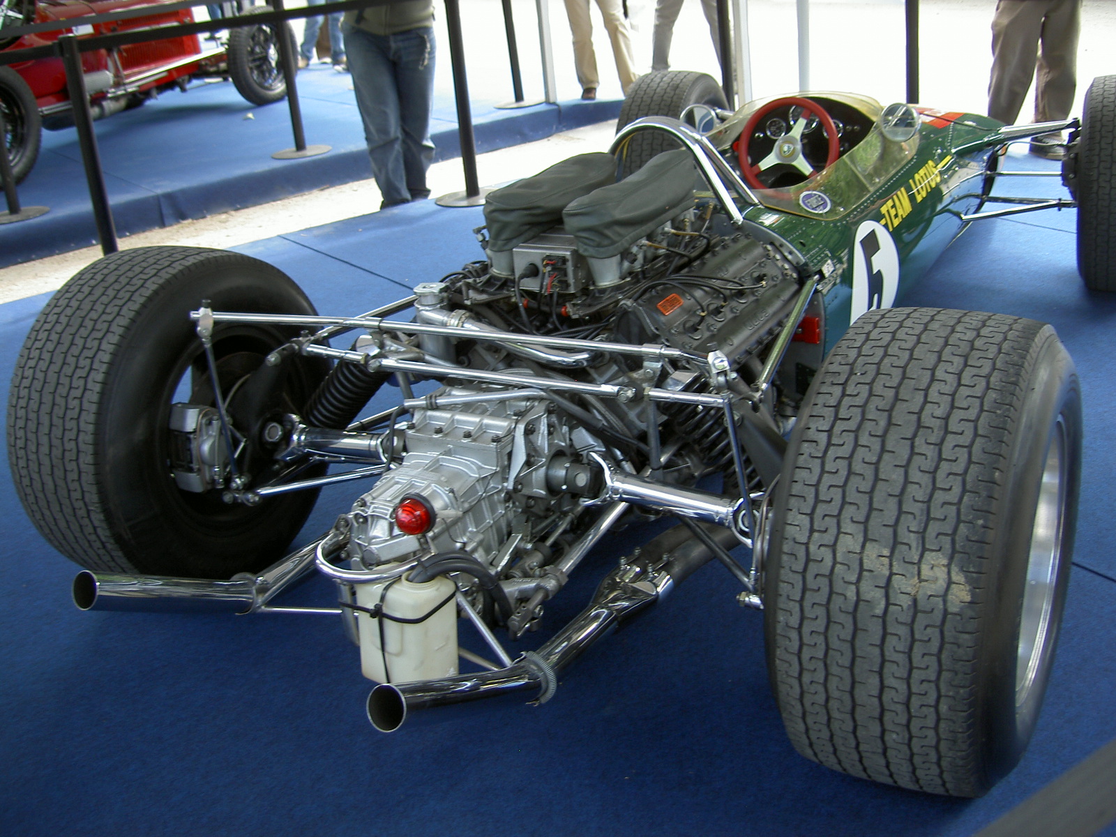
Figure: The Lotus 49, view from the rear. The Lotus 49 was one of the last Formula One cars before the introduction of aerodynamic aids.

So when it comes to our ability to compute we are extraordinary, not compute in our conscious mind, but the underlying neuron firings that underpin both our consciousness, our subconsciousness as well as our motor control etc.

If we think of ourselves as vehicles, then we are massively overpowered. Our ability to generate derived information from raw fuel is extraordinary. Intellectually we have formula one engines.

But in terms of our ability to deploy that computation in actual use, to share the results of what we have inferred, we are very limited. So when you imagine the F1 car that represents a psyche, think of an F1 car with bicycle wheels.

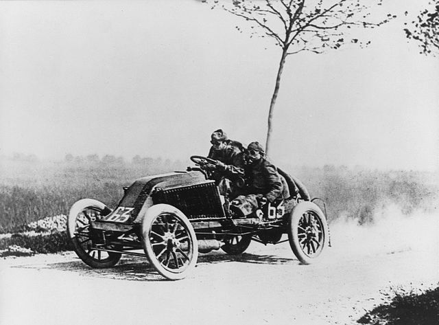
Figure: Marcel Renault races a Renault 40 cv during the Paris-Madrid race, an early Grand Prix, in 1903. Marcel died later in the race after missing a warning flag for a sharp corner at Couhé Vérac, likely due to dust reducing visibility.

Just think of the control a driver would have to have to deploy such power through such a narrow channel of traction. That is the beauty and the skill of the human mind.

In contrast, our computers are more like go-karts. Underpowered, but with well-matched tires. They can communicate far more fluidly. They are more efficient, but somehow less extraordinary, less beautiful.

Figure: Caleb McDuff driving for WIX Silence Racing.

For humans, that means much of our computation should be dedicated to considering what we should compute. To do that efficiently we need to model the world around us. The most complex thing in the world around us is other humans. So it is no surprise that we model them. We second guess what their intentions are, and our communication is only necessary when they are departing from how we model them. Naturally, for this to work well, we need to understand those we work closely with. So it is no surprise that social communication, social bonding, forms so much of a part of our use of our limited bandwidth.

There is a second effect here, our need to anthropomorphise objects around us. Our tendency to model our fellow humans extends to when we interact with other entities in our environment. To our pets as well as inanimate objects around us, such as computers or even our cars. This tendency to over interpret could be a consequence of our limited ability to communicate.²

For more details see this paper “Living Together: Mind and Machine Intelligence”, and this TEDx talk.

Evolved Relationship with Information

The high bandwidth of computers has resulted in a close relationship between the computer and data. Large amounts of information can flow between the two. The degree to which the computer is mediating our relationship with data means that we should consider it an intermediary.

Originaly our low bandwith relationship with data was affected by two characteristics. Firstly, our tendency to over-interpret driven by our need to extract as much knowledge from our low bandwidth information channel as possible. Secondly, by our improved understanding of the domain of mathematical statistics and how our cognitive biases can mislead us.

With this new set up there is a potential for assimilating far more information via the computer, but the computer can present this to us in various ways. If it’s motives are not aligned with ours then it can misrepresent the information. This needn’t be nefarious it can be simply as a result of the computer pursuing a different objective from us. For example, if the computer is aiming to maximize our interaction time that may be a different objective from ours which may be to summarize information in a representative manner in the shortest possible length of time.

For example, for me, it was a common experience to pick up my telephone with the intention of checking when my next appointment was, but to soon find myself distracted by another application on the phone, and end up reading something on the internet. By the time I’d finished reading, I would often have forgotten the reason I picked up my phone in the first place.

There are great benefits to be had from the huge amount of information we can unlock from this evolved relationship between us and data. In biology, large scale data sharing has been driven by a revolution in genomic, transcriptomic and epigenomic measurement. The improved inferences that can be drawn through summarizing data by computer have fundamentally changed the nature of biological science, now this phenomenon is also infuencing us in our daily lives as data measured by happenstance is increasingly used to characterize us.

Better mediation of this flow actually requires a better understanding of human-computer interaction. This in turn involves understanding our own intelligence better, what its cognitive biases are and how these might mislead us.

For further thoughts see Guardian article on marketing in the internet era from 2015.

You can also check my blog post on System Zero. also from 2015.

New Flow of Information

Classically the field of statistics focussed on mediating the relationship between the machine and the human. Our limited bandwidth of communication means we tend to over-interpret the limited information that we are given, in the extreme we assign motives and desires to inanimate objects (a process known as anthropomorphizing). Much of mathematical statistics was developed to help temper this tendency and understand when we are valid in drawing conclusions from data.

Figure: The trinity of human, data and computer, and highlights the modern phenomenon. The communication channel between computer and data now has an extremely high bandwidth. The channel between human and computer and the channel between data and human is narrow. New direction of information flow, information is reaching us mediated by the computer. The focus on classical statistics reflected the importance of the direct communication between human and data. The modern challenges of data science emerge when that relationship is being mediated by the machine.

Data science brings new challenges. In particular, there is a very large bandwidth connection between the machine and data. This means that our relationship with data is now commonly being mediated by the machine. Whether this is in the acquisition of new data, which now happens by happenstance rather than with purpose, or the interpretation of that data where we are increasingly relying on machines to summarise what the data contains. This is leading to the emerging field of data science, which must not only deal with the same challenges that mathematical statistics faced in tempering our tendency to over interpret data, but must also deal with the possibility that the machine has either inadvertently or malisciously misrepresented the underlying data.

What does Machine Learning do?

Any process of automation allows us to scale what we do by codifying a process in some way that makes it efficient and repeatable. Machine learning automates by emulating human (or other actions) found in data. Machine learning codifies in the form of a mathematical function that is learnt by a computer. If we can create these mathematical functions in ways in which they can interconnect, then we can also build systems.

Machine learning works through codifing a prediction of interest into a mathematical function. For example, we can try and predict the probability that a customer wants to by a jersey given knowledge of their age, and the latitude where they live. The technique known as logistic regression estimates the odds that someone will by a jumper as a linear weighted sum of the features of interest.

\[ \text{odds} = \frac{p(\text{bought})}{p(\text{not bought})} \]

\[ \log \text{odds} = \beta_0 + \beta_1 \text{age} + \beta_2 \text{latitude}.\] Here \(\beta_0\), \(\beta_1\) and \(\beta_2\) are the parameters of the model. If \(\beta_1\) and \(\beta_2\) are both positive, then the log-odds that someone will buy a jumper increase with increasing latitude and age, so the further north you are and the older you are the more likely you are to buy a jumper. The parameter \(\beta_0\) is an offset parameter, and gives the log-odds of buying a jumper at zero age and on the equator. It is likely to be negative³ indicating that the purchase is odds-against. This is actually a classical statistical model, and models like logistic regression are widely used to estimate probabilities from ad-click prediction to risk of disease.

This is called a generalized linear model, we can also think of it as estimating the probability of a purchase as a nonlinear function of the features (age, lattitude) and the parameters (the \(\beta\) values). The function is known as the sigmoid or logistic function, thus the name logistic regression.

\[ p(\text{bought}) = \sigma\left(\beta_0 + \beta_1 \text{age} + \beta_2 \text{latitude}\right).\] In the case where we have features to help us predict, we sometimes denote such features as a vector, \(\mathbf{ x}\), and we then use an inner product between the features and the parameters, \(\boldsymbol{\beta}^\top \mathbf{ x}= \beta_1 x_1 + \beta_2 x_2 + \beta_3 x_3 ...\), to represent the argument of the sigmoid.

\[ p(\text{bought}) = \sigma\left(\boldsymbol{\beta}^\top \mathbf{ x}\right).\] More generally, we aim to predict some aspect of our data, \(y\), by relating it through a mathematical function, \(f(\cdot)\), to the parameters, \(\boldsymbol{\beta}\) and the data, \(\mathbf{ x}\).

\[ y= f\left(\mathbf{ x}, \boldsymbol{\beta}\right).\] We call \(f(\cdot)\) the prediction function.

To obtain the fit to data, we use a separate function called the objective function that gives us a mathematical representation of the difference between our predictions and the real data.

\[E(\boldsymbol{\beta}, \mathbf{Y}, \mathbf{X})\] A commonly used examples (for example in a regression problem) is least squares, \[E(\boldsymbol{\beta}, \mathbf{Y}, \mathbf{X}) = \sum_{i=1}^n\left(y_i - f(\mathbf{ x}_i, \boldsymbol{\beta})\right)^2.\]

If a linear prediction function is combined with the least squares objective function then that gives us a classical linear regression, another classical statistical model. Statistics often focusses on linear models because it makes interpretation of the model easier. Interpretation is key in statistics because the aim is normally to validate questions by analysis of data. Machine learning has typically focussed more on the prediction function itself and worried less about the interpretation of parameters, which are normally denoted by \(\mathbf{w}\) instead of \(\boldsymbol{\beta}\). As a result non-linear functions are explored more often as they tend to improve quality of predictions but at the expense of interpretability.

Deep Learning

Classical statistical models and simple machine learning models have a great deal in common. The main difference between the fields is philosophical. Machine learning practitioners are typically more concerned with the quality of prediciton (e.g. measured by ROC curve) while statisticians tend to focus more on the interpretability of the model and the validity of any decisions drawn from that interpretation. For example, a statistical model may be used to validate whether a large scale intervention (such as the mass provision of mosquito nets) has had a long term effect on disease (such as malaria). In this case one of the covariates is likely to be the provision level of nets in a particular region. The response variable would be the rate of malaria disease in the region. The parmaeter, \(\beta_1\) associated with that covariate will demonstrate a positive or negative effect which would be validated in answering the question. The focus in statistics would be less on the accuracy of the response variable and more on the validity of the interpretation of the effect variable, \(\beta_1\).

A machine learning practitioner on the other hand would typically denote the parameter \(w_1\), instead of \(\beta_1\) and would only be interested in the output of the prediction function, \(f(\cdot)\) rather than the parameter itself. The general formalism of the prediction function allows for non-linear models. In machine learning, the emphasis on prediction over interpretability means that non-linear models are often used. The parameters, \(\mathbf{w}\), are a means to an end (good prediction) rather than an end in themselves (interpretable).

DeepFace

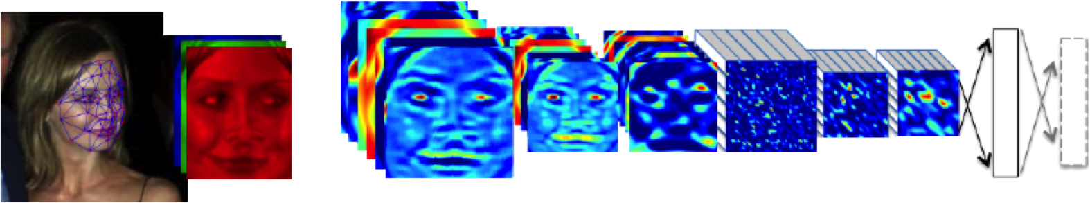
Figure: The DeepFace architecture (Taigman et al., 2014), visualized through colors to represent the functional mappings at each layer. There are 120 million parameters in the model.

The DeepFace architecture (Taigman et al., 2014) consists of layers that deal with translation invariances, known as convolutional layers. These layers are followed by three locally-connected layers and two fully-connected layers. Color illustrates feature maps produced at each layer. The neural network includes more than 120 million parameters, where more than 95% come from the local and fully connected layers.

Deep Learning as Pinball

Figure: Deep learning models are composition of simple functions. We can think of a pinball machine as an analogy. Each layer of pins corresponds to one of the layers of functions in the model. Input data is represented by the location of the ball from left to right when it is dropped in from the top. Output class comes from the position of the ball as it leaves the pins at the bottom.

Sometimes deep learning models are described as being like the brain, or too complex to understand, but one analogy I find useful to help the gist of these models is to think of them as being similar to early pin ball machines.

In a deep neural network, we input a number (or numbers), whereas in pinball, we input a ball.

Think of the location of the ball on the left-right axis as a single number. Our simple pinball machine can only take one number at a time. As the ball falls through the machine, each layer of pins can be thought of as a different layer of ‘neurons.’ Each layer acts to move the ball from left to right.

In a pinball machine, when the ball gets to the bottom it might fall into a hole defining a score, in a neural network, that is equivalent to the decision: a classification of the input object.

An image has more than one number associated with it, so it is like playing pinball in a hyper-space.

Figure: At initialization, the pins, which represent the parameters of the function, aren’t in the right place to bring the balls to the correct decisions.

Figure: After learning the pins are now in the right place to bring the balls to the correct decisions.

Learning involves moving all the pins to be in the correct position, so that the ball ends up in the right place when it’s fallen through the machine. But moving all these pins in hyperspace can be difficult.

In a hyper-space you have to put a lot of data through the machine for to explore the positions of all the pins. Even when you feed many millions of data points through the machine, there are likely to be regions in the hyper-space where no ball has passed. When future test data passes through the machine in a new route unusual things can happen.

Adversarial examples exploit this high dimensional space. If you have access to the pinball machine, you can use gradient methods to find a position for the ball in the hyper space where the image looks like one thing, but will be classified as another.

Probabilistic methods explore more of the space by considering a range of possible paths for the ball through the machine. This helps to make them more data efficient and gives some robustness to adversarial examples.

Data Science and Professionalisation

The rise in data science and artificial intelligence technologies has been termed “Industrial Revolution 4.0,” so are we in the midst of an industrial change? Maybe, but if so, it is the first part of the industrial revolution to be named before it has happened. The original industrial revolution occurred between 1760 and 1840, but the term was introduced into English by Arnold Toynbee (1852-1883).

Whether this is a new revolution or an extension of previous revolutions, an important aspect is that this revolution is dominated by data instead of just capital.

One can also see the modern revolution as a revolution in information rather than energy.

Disruptive technologies take time to assimilate, and best practices, as well as the pitfalls of new technologies take time to share. Historically, new technologies led to new professions. Isambard Kingdom Brunel (born 1806) was a leading innovator in civil, mechanical and naval engineering. Each of these has its own professional institutions founded in 1818, 1847, and 1860 respectively.

Nikola Tesla developed the modern approach to electrical distribution, he was born in 1856 and the American Instiute for Electrical Engineers was founded in 1884, the UK equivalent was founded in 1871.

William Schockley Jr, born 1910, led the group that developed the transistor, referred to as “the man who brought silicon to Silicon Valley,” in 1963 the American Institute for Electical Engineers merged with the Institute of Radio Engineers to form the Institute of Electrical and Electronic Engineers.

Watts S. Humphrey, born 1927, was known as the “father of software quality,” in the 1980s he founded a program aimed at understanding and managing the software process. The British Computer Society was founded in 1956.

Why the need for these professions? Much of it is about codification of best practice and developing trust between the public and practitioners. These fundamental characteristics of the professions are shared with the oldest professions (Medicine, Law) as well as the newest (Information Technology).

So where are we today? My best guess is we are somewhere equivalent to the 1980s for Software Engineering. In terms of professional deployment we have a basic understanding of the equivalent of “programming” but much less understanding of machine learning systems design and data infrastructure. How the components we ahve developed interoperate together in a reliable and accountable manner. Best practice is still evolving, but perhaps isn’t being shared widely enough.

One problem is that the art of data science is superficially similar to regular software engineering. Although in practice it is rather different. Modern software engineering practice operates to generate code which is well tested as it is written, agile programming techniques provide the appropriate degree of flexibility for the individual programmers alongside sufficient formalization and testing. These techniques have evolved from an overly restrictive formalization that was proposed in the early days of software engineering.

While data science involves programming, it is different in the following way. Most of the work in data science involves understanding the data and the appropriate manipulations to apply to extract knowledge from the data. The eventual number of lines of code that are required to extract that knowledge are often very few, but the amount of thought and attention that needs to be applied to each line is much more than a traditional line of software code. Testing of those lines is also of a different nature, provisions have to be made for evolving data environments. Any development work is often done on a static snapshot of data, but deployment is made in a live environment where the nature of data changes. Quality control involves checking for degradation in performance arising form unanticipated changes in data quality. It may also need to check for regulatory conformity. For example, in the UK the General Data Protection Regulation stipulates standards of explainability and fairness that may need to be monitored. These concerns do not affect traditional software deployments.

Others are also pointing out these challenges, this post from Andrej Karpathy (now head of AI at Tesla) covers the notion of “Software 2.0.” Google researchers have highlighted the challenges of “Technical Debt” in machine learning (Sculley et al., 2015). Researchers at Berkeley have characterized the systems challenges associated with machine learning (Stoica et al., 2017).

The Data Crisis

Anecdotally, talking to data modelling scientists. Most say they spend 80% of their time acquiring and cleaning data. This is precipitating what I refer to as the “data crisis.” This is an analogy with software. The “software crisis” was the phenomenon of inability to deliver software solutions due to increasing complexity of implementation. There was no single shot solution for the software crisis, it involved better practice (scrum, test orientated development, sprints, code review), improved programming paradigms (object orientated, functional) and better tools (CVS, then SVN, then git).

However, these challenges aren’t new, they are merely taking a different form. From the computer’s perspective software is data. The first wave of the data crisis was known as the software crisis.

The Software Crisis

In the late sixties early software programmers made note of the increasing costs of software development and termed the challenges associated with it as the “Software Crisis.” Edsger Dijkstra referred to the crisis in his 1972 Turing Award winner’s address.

The major cause of the software crisis is that the machines have become several orders of magnitude more powerful! To put it quite bluntly: as long as there were no machines, programming was no problem at all; when we had a few weak computers, programming became a mild problem, and now we have gigantic computers, programming has become an equally gigantic problem.

Edsger Dijkstra (1930-2002), The Humble Programmer

The major cause of the data crisis is that machines have become more interconnected than ever before. Data access is therefore cheap, but data quality is often poor. What we need is cheap high-quality data. That implies that we develop processes for improving and verifying data quality that are efficient.

There would seem to be two ways for improving efficiency. Firstly, we should not duplicate work. Secondly, where possible we should automate work.

What I term “The Data Crisis” is the modern equivalent of this problem. The quantity of modern data, and the lack of attention paid to data as it is initially “laid down” and the costs of data cleaning are bringing about a crisis in data-driven decision making. This crisis is at the core of the challenge of technical debt in machine learning (Sculley et al., 2015).

Just as with software, the crisis is most correctly addressed by ‘scaling’ the manner in which we process our data. Duplication of work occurs because the value of data cleaning is not correctly recognised in management decision making processes. Automation of work is increasingly possible through techniques in “artificial intelligence,” but this will also require better management of the data science pipeline so that data about data science (meta-data science) can be correctly assimilated and processed. The Alan Turing institute has a program focussed on this area, AI for Data Analytics.

• Reusability of Data

• Deployment of Machine Learning Systems

Data Readiness Levels

Data Readiness Levels

Data Readiness Levels (Lawrence, 2017b) are an attempt to develop a language around data quality that can bridge the gap between technical solutions and decision makers such as managers and project planners. They are inspired by Technology Readiness Levels which attempt to quantify the readiness of technologies for deployment.

See this blog post on Data Readiness Levels.

Three Grades of Data Readiness

Data-readiness describes, at its coarsest level, three separate stages of data graduation.

• Grade C - accessibility
  • Transition: data becomes electronically available
• Grade B - validity
  • Transition: pose a question to the data.
• Grade A - usability

The important definitions are at the transition. The move from Grade C data to Grade B data is delimited by the electronic availability of the data. The move from Grade B to Grade A data is delimited by posing a question or task to the data (Lawrence:drl17?).

Accessibility: Grade C

The first grade refers to the accessibility of data. Most data science practitioners will be used to working with data-providers who, perhaps having had little experience of data-science before, state that they “have the data.” More often than not, they have not verified this. A convenient term for this is “Hearsay Data,” someone has heard that they have the data so they say they have it. This is the lowest grade of data readiness.

Progressing through Grade C involves ensuring that this data is accessible. Not just in terms of digital accessiblity, but also for regulatory, ethical and intellectual property reasons.

Validity: Grade B

Data transits from Grade C to Grade B once we can begin digital analysis on the computer. Once the challenges of access to the data have been resolved, we can make the data available either via API, or for direct loading into analysis software (such as Python, R, Matlab, Mathematica or SPSS). Once this has occured the data is at B4 level. Grade B involves the validity of the data. Does the data really represent what it purports to? There are challenges such as missing values, outliers, record duplication. Each of these needs to be investigated.

Grade B and C are important as if the work done in these grades is documented well, it can be reused in other projects. Reuse of this labour is key to reducing the costs of data-driven automated decision making. There is a strong overlap between the work required in this grade and the statistical field of exploratory data analysis (Tukey, 1977).

The need for Grade B emerges due to the fundamental change in the availability of data. Classically, the scientific question came first, and the data came later. This is still the approach in a randomized control trial, e.g. in A/B testing or clinical trials for drugs. Today data is being laid down by happenstance, and the question we wish to ask about the data often comes after the data has been created. The Grade B of data readiness ensures thought can be put into data quality before the question is defined. It is this work that is reusable across multiple teams. It is these processes that the team which is standing up the data must deliver.

Usability: Grade A

Once the validity of the data is determined, the data set can be considered for use in a particular task. This stage of data readiness is more akin to what machine learning scientists are used to doing in Universities. Bringing an algorithm to bear on a well understood data set.

In Grade A we are concerned about the utility of the data given a particular task. Grade A may involve additional data collection (experimental design in statistics) to ensure that the task is fulfilled.

This is the stage where the data and the model are brought together, so expertise in learning algorithms and their application is key. Further ethical considerations, such as the fairness of the resulting predictions are required at this stage. At the end of this stage a prototype model is ready for deployment.

Deployment and maintenance of machine learning models in production is another important issue which Data Readiness Levels are only a part of the solution for.

Recursive Effects

To find out more, or to contribute ideas go to http://data-readiness.org

Throughout the data preparation pipeline, it is important to have close interaction between data scientists and application domain experts. Decisions on data preparation taken outside the context of application have dangerous downstream consequences. This provides an additional burden on the data scientist as they are required for each project, but it should also be seen as a learning and familiarization exercise for the domain expert. Long term, just as biologists have found it necessary to assimilate the skills of the bioinformatician to be effective in their science, most domains will also require a familiarity with the nature of data driven decision making and its application. Working closely with data-scientists on data preparation is one way to begin this sharing of best practice.

The processes involved in Grade C and B are often badly taught in courses on data science. Perhaps not due to a lack of interest in the areas, but maybe more due to a lack of access to real world examples where data quality is poor.

These stages of data science are also ridden with ambiguity. In the long term they could do with more formalization, and automation, but best practice needs to be understood by a wider community before that can happen.

Assessing the Organizations Readiness

Assessing the readiness of data for analysis is one action that can be taken, but assessing teams that need to assimilate the information in the data is the other side of the coin. With this in mind both Damon Civin and Nick Elprin have independently proposed the idea of a “Data Joel Test.” A “Joel Test” is a short questionaire to establish the ability of a team to handle software engineering tasks. It is designed as a rough and ready capability assessment. A “Data Joel Test” is similar, but for assessing the capability of a team in performing data science.

Deploying Artificial Intelligence

With the wide availability of new techniques, we are currently creating Artifical Intelligence through combination of machine learning algorithms to form machine learning systems.

This effect is amplified through the growth in sensorics, in particular the movement of cloud computing towards the customer. The barrier between cloud and device is blurring. This phenomenon is sometimes known as fog computing, or computing on the edge.

This presents major new challenges for machine learning systems design. We would like an internet of intelligence but currently our AI systems are fragile. A classical systems approach to design does not handle evolving environments well.

Machine Learning Systems Design

The challenges of integrating different machine learning components into a whole that acts effectively as a system seem unresolved. In software engineering, separating parts of a system in this way is known as component-based software engineering. The core idea is that the different parts of the system can be independently designed according to a sub-specfication. This is sometimes known as separation of concerns. However, once the components are machine learning based, tighter coupling becomes a side effect of the learned nature of the system. For example if a driverless car’s detection of cyclist is dependent on its detection of the road surface, a change in the road surface detection algorithm will have downstream effects on the cyclist detection. Even if the road detection system has been improved by objective measures, the cyclist detection system may have become sensitive to the foibles of the previous version of road detection and will need to be retrained.

Most of our experience with deployment relies on some approximation to the component based model, this is also important for verification of the system. If the components of the system can be verified then the composed system can also, potentially, be verified.

Pigeonholing

Figure: Decompartmentalization of the model into parts can be seen as pigeonholing the separate tasks that are required.

To deal with the complexity of systems design, a common approach is to break complex systems down into a series of tasks. An approach we can think of as “pigeonholing.” Classically, a sub-task could be thought of as a particular stage in machining (by analogy to productionlines in factories) or a sub-routine call in computing. Machine learning allows any complex sub-task, that was difficult to decompose by classical methods, to be reconstituted by acquiring data. In particular, when we think of emulating a human, we can ask many humans to perform the sub-task many times and fit machine learning models to reconstruct the performance, or to emulate the human in the performance of the task. For example, the decomposition of a complex process such as driving a car into apparently obvious sub-tasks (following the road, identifying pedestrians, etc).

The practitioner’s approach to deploying artificial intelligence systems is to build up systems of machine learning components. To build a machine learning system, we decompose the task into parts, each of which we can emulate with ML methods. These parts are typically independently constructed and verified. For example, in a driverless car we can decompose the tasks into components such as “pedestrian detection” and “road line detection.” Each of these components can be constructed with, for example, a classification algorithm. Nowadays, people will often deploy a deep neural network, but for many tasks a random forest algorithm may be sufficient. We can then superimpose a logic on top. For example, “Follow the road line unless you detect a pedestrian in the road.”

This allows for verification of car performance, as long as we can verify the individual components. However, it also implies that the AI systems we deploy are fragile.

Our intelligent systems are composed by “pigeonholing” each indvidual task, then substituting with a machine learning model.

But this is not a robust approach to systems design. The definition of sub-tasks can lead to a single point of failure, where if any sub-task fails, the entire system fails.

Rapid Reimplementation

This is also the classical approach to automation, but in traditional automation we also ensure the environment in which the system operates becomes controlled. For example, trains run on railway lines, fast cars run on motorways, goods are manufactured in a controlled factory environment.

The difference with modern automated decision making systems is our intention is to deploy them in the uncontrolled environment that makes up our own world.

This exposes us to either unforseen circumstances or adversarial action. And yet it is unclear our our intelligent systems are capable of adapting to this.

We become exposed to mischief and adversaries. Adversaries intentially may wish to take over the artificial intelligence system, and mischief is the constant practice of many in our society. Simply watching a 10 year old interact with a voice agent such as Alexa or Siri shows that they are delighted when the can make the the “intelligent” agent seem foolish.

The Centrifugal Governor

Figure: Centrifugal governor as held by “Science” on Holborn Viaduct

Boulton and Watt’s Steam Engine

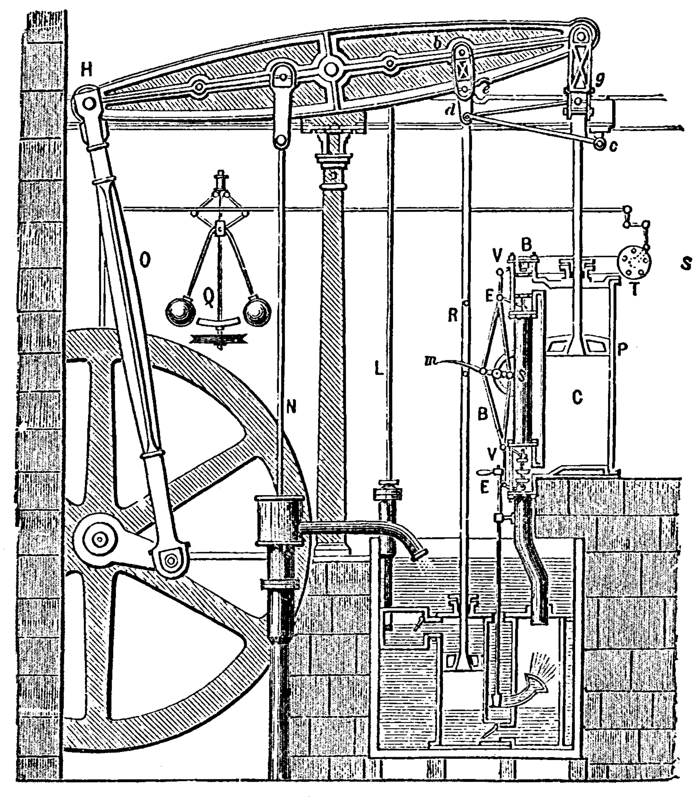
Figure: Watt’s Steam Engine which made Steam Power Efficient and Practical.

James Watt’s steam engine contained an early machine learning device. In the same way that modern systems are component based, his engine was composed of components. One of which is a speed regulator sometimes known as Watt’s governor. The two balls in the center of the image, when spun fast, rise, and through a linkage mechanism.

The centrifugal governor was made famous by Boulton and Watt when it was deployed in the steam engine. Studying stability in the governor is the main subject of James Clerk Maxwell’s paper on the theoretical analysis of governors (Maxwell, 1867). This paper is a founding paper of control theory. In an acknowledgment of its influence, Wiener used the name cybernetics to describe the field of control and communication in animals and the machine (Wiener, 1948). Cybernetics is the Greek word for governor, which comes from the latin for helmsman.

A governor is one of the simplest artificial intelligence systems. It senses the speed of an engine, and acts to change the position of the valve on the engine to slow it down.

Although it’s a mechanical system a governor can be seen as automating a role that a human would have traditionally played. It is an early example of artificial intelligence.

The centrifugal governor has several parameters, the weight of the balls used, the length of the linkages and the limits on the balls movement.

Two principle differences exist between the centrifugal governor and artificial intelligence systems of today.

1. The centrifugal governor is a physical system and it is an integral part of a wider physical system that it regulates (the engine).
2. The parameters of the governor were set by hand, our modern artificial intelligence systems have their parameters set by data.

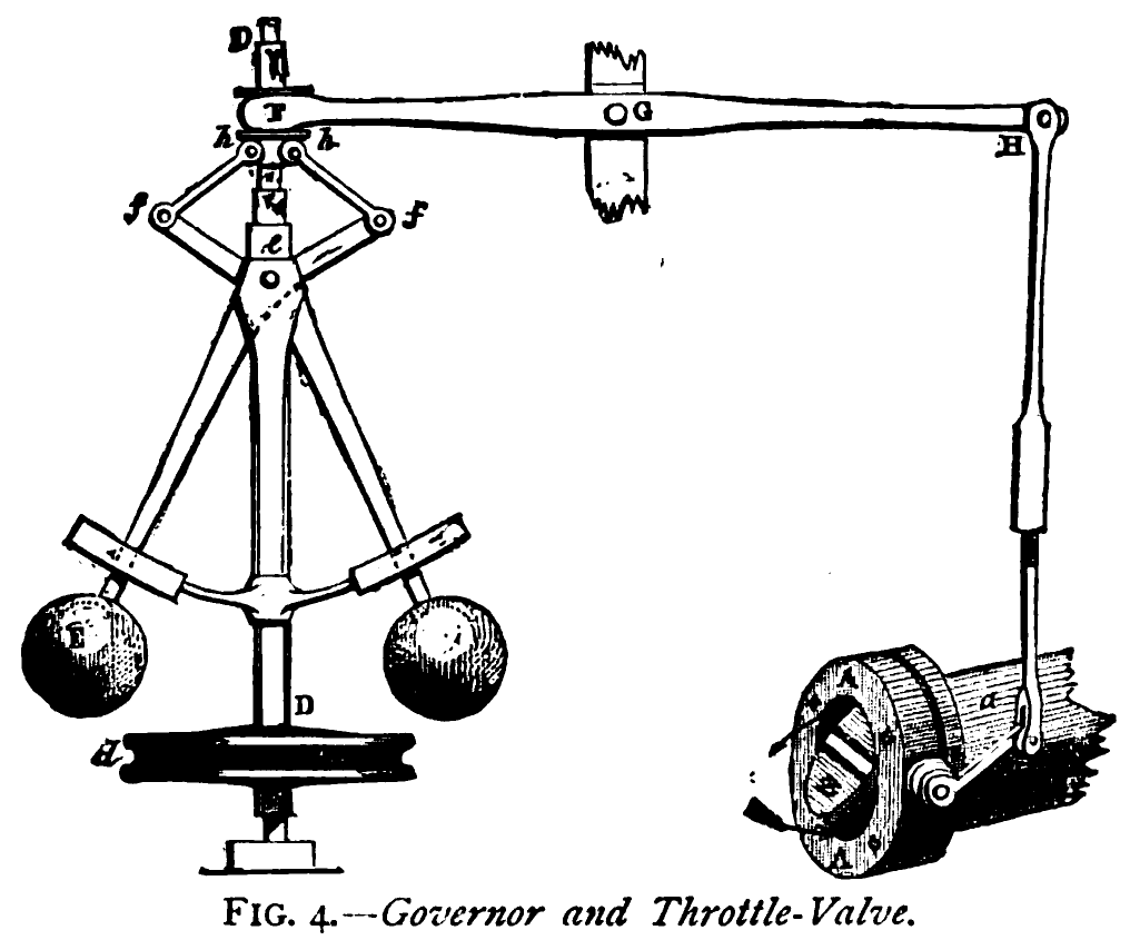
Figure: The centrifugal governor, an early example of a decision making system. The parameters of the governor include the lengths of the linkages (which effect how far the throttle opens in response to movement in the balls), the weight of the balls (which effects inertia) and the limits of to which the balls can rise.

This has the basic components of sense and act that we expect in an intelligent system, and this system saved the need for a human operator to manually adjust the system in the case of overspeed. Overspeed has the potential to destroy an engine, so the governor operates as a safety device.

The first wave of automation did bring about sabotoage as a worker’s response. But if machinery was sabotaged, for example, if the linkage between sensor (the spinning balls) and action (the valve closure) was broken, this would be obvious to the engine operator at start up time. The machine could be repaired before operation.

The centrifugal governor was a key component in the Boulton-Watt steam engine. It senses increases in speed in the engine and closed the steam valve to prevent the engine overspeeding and destroying itself. Until the invention of this device, it was a human job to do this.

The formal study of governors and other feedback control devices was then began by James Clerk Maxwell, the Scottish physicist. This field became the foundation of our modern techniques of artificial intelligence through Norbert Wiener’s book Cybernetics (Wiener, 1948). Cybernetics is Greek for governor, a word that in itself simply means helmsman in English.

The recent WannaCry virus that had a wide impact on our health services ecosystem was exploiting a security flaw in Windows systems that was first exploited by a virus called Stuxnet.

Stuxnet was a virus designed to infect the Iranian nuclear program’s Uranium enrichment centrifuges. A centrifuge is prevented from overspeed by a controller, just like the centrifugal governor. Only now it is implemented in control logic, in this case on a Siemens PLC controller.

Stuxnet infected these controllers and took over the response signal in the centrifuge, fooling the system into thinking that no overspeed was occuring. As a result, the centrifuges destroyed themselves through spinning too fast.

This is equivalent to detaching the governor from the steam engine. Such sabotage would be easily recognized by a steam engine operator. The challenge for the operators of the Iranian Uranium centrifuges was that the sabotage was occurring inside the electronics.

That is the effect of an adversary on an intelligent system, but even without adveraries, the mischief of a 10 year old can confuse our AIs.

Peppercorns

Figure: A peppercorn is a system design failure which is not a bug, but a conformance to design specification that causes problems when the system is deployed in the real world with mischevious and adversarial actors.

Asking Siri “What is a trillion to the power of a thousand minus one?” leads to a 30 minute response⁴ consisting of only 9s. I found this out because my nine year old grabbed my phone and did it. The only way to stop Siri was to force closure. This is an interesting example of a system feature that’s not a bug, in fact it requires clever processing from Wolfram Alpha. But it’s an unexpected result from the system performing correctly.

This challenge of facing a circumstance that was unenvisaged in design but has consequences in deployment becomes far larger when the environment is uncontrolled. Or in the extreme case, where actions of the intelligent system effect the wider environment and change it.

These unforseen circumstances are likely to lead to need for much more efficient turn-around and update for our intelligent systems. Whether we are correcting for security flaws (which are bugs) or unenvisaged circumstantial challenges: an issue I’m referring to as peppercorns. Rapid deployment of system updates is required. For example, Apple have “fixed” the problem of Siri returning long numbers.

Here’s another one from Reddit, of a Tesla Model 3 system hallucinating traffic lights.

The challenge is particularly acute because of the scale at which we can deploy AI solutions. This means when something does go wrong, it may be going wrong in billions of households simultaneously.

You can also check this blog post on Decision Making and Diversity. and this blog post on Natural vs Artifical Intelligence..

Conclusion

Artificial Intelligence and Data Science are fundamentally different. In one you are dealing with data collected by happenstance. In the other you are trying to build systems in the real world, often by actively collecting data. Our approaches to systems design are building powerful machines that will be deployed in evolving environments. There is an urgent need for new ideas and methodologies for safe deployment and redployment of these systems.

Thanks!

For more information on these subjects and more you might want to check the following resources.

• twitter: @lawrennd

• podcast: The Talking Machines

• newspaper: Guardian Profile Page

• blog posts:

• Andrej Karpathy’s Medium Post

• Mike Jordan’s Medium Post

References