Information, Energy and Intelligence
Abstract
David MacKay’s work emphasized explicit assumptions and operational clarity in modeling information and inference. In games like Conway’s Life, rules are explicit and self-contained. In analytic frameworks, we often take implicit adjudicators for granted—external observers, pre-specified outcome spaces, privileged decompositions. What if we forbid such external adjudication and seek only rules that can be applied from within the system?
This talk explores the “inaccessible game,” an information-theoretic dynamical system where all rules must be internally adjudicable. Starting from three axioms characterizing information loss (Baez-Fritz-Leinster), we show how a “no-barber principle” selects marginal entropy conservation, maximum entropy dynamics, and specific substrate properties, not by assumption but by consistency requirements. We explore when the constraints imply energy-entropy equivalence in the thermodynamic limit and how entropy time becomes a distinguished clock withn the framework.
This work is dedicated to the memory of David MacKay.
In Memory of David MacKay
This talk is for a memorial meeting for David MacKay, who made fundamental contributions to our understanding of the relationship between information theory, energy, and practical systems. David’s work on information theory and inference provided elegant bridges between abstract mathematical principles and real-world applications.
I first saw David speak about information theory at the 1997 Issac Newton Institute meeting on Machine Learning and Genaralisation. It was a suprise because I had been expecting him to speak about either Bayesian neural networks or Gaussian processes. But, of course, as you get to know David you realise it was unsurprising, because he’d been looking at the connections between information theory, machine learning and error correcting codes. He summarised his thinking in his book “Information Theory, Inference, and Learning Algorithms” (MacKay, 2003). It demonstrated how information-theoretic thinking can illuminate everything from error-correcting codes to neural networks to sexual reproduction. This book was my introduction to information theory, and it was available long before it was published. Regular updates were made on David’s website from the late 1990s.
He later surprised me again, when I heard that he’d shifted away from this larger work and was focussing on energy. He did so because he believed that sustainable energy was the most important challenge humanity faced. He approache the subject with the same clarity of thinking and careful reasoning. Memorably underpinned by practical examples using phone chargers. “Sustainable Energy Without the Hot Air” (MacKay, 2008) was published in 2008. In a video created as part of the 2009 Cambridge Campaign he went from phone chargers to sweeping national changes in the way we use energy.

Figure: A YouTube video featuring David’s clarity of thought and the ideas behind sustainable energy from 2010.
This Talk
The work I present today on the inaccessible game is my best attempt to follow in this tradition. It tries to build on rigorous information-theoretic foundations for understanding the limitations of automotous information systems. The hope is to use this framework to underpin our understanding of information processing systems, what their limits are. I hope that David would have appreciated both the mathematical structure and the attempt to use it to deflate unrealistic promises about superintelligence which I see as problematic in the same way he felt conversations about phone chargers were problematic in distracting us from the real challenges of energy restructuring.
As David told us ten years ago, he was highly inspired by John Bridle telling him (as an undergraduate student) “everything’s connected.” Across his workDavid taught us to ask: “What are the fundamental constraints? What do the numbers say?”
In my best attempt to respect that spirit of inquiry, this work tries to ask: What fundamental information-theoretic constraints govern intelligent systems? Can we understand these constraints as rigorously as we understand thermodynamic constraints on engines?
Ultimate
David was also a playful person, he enjoyed games, often rephrasing physics questions as puzzles, but also ultimate frisbee,1 or ultimate for short. One aspect of ultimate he seemed to particularly like was the “spirit of the game.” In ultimate there is no referee, no arbitration. Self arbitration is part of the spirit of the game.

In honour of this idea, we consider a similar principle for “zero player games.” Games of the type of Conway’s game of life (Gardner (1970)) or Wolfram’s cellular automata (Wolfram (1983)). The principle is a conceptual constraint inspired by Russell’s paradox: it demands that the rules of our system not appeal to external adjudicators or reference points just like ultimate.
The Munchkin Provision
Without such consistency, we would require what we might call a “Munchkin provision.” In the Munchkin card game (Jackson, 2001), it is acknowledged that the cards and rules may be inconsistent. Their resolution?
Any other disputes should be settled by loud arguments, with the owner of the game having the last word.
Munckin Rules (Jackson, 2001)
While this works for card games, it’s unsatisfying for foundational mathematics. We want our game to be internally consistent, not requiring an external referee to resolve paradoxes.

Figure: The Munchkin card came has both cards and rules. The game explicitly acknowledges that this can lead to inconsistencies which should be resolved by the game owner.
A Tautology
Self-governing systems cannot refer to external arbitration.
While this is a tautology, we’re going to try and suggest how to formalise this notion. Given that this is a memorial to David, we’re going to look to define it through information theory.
When I arrived in Cambridge in February 1998, David was already working on coding and his meetings consisted of discussions of information theory, which was new to me. My background was as a Mechanical Engineer, and what I had learnt about Bayesian probability came from a terms preparation for my PhD at Aston University.
David’s lectures consisted of discussions of Shannon limits and low density parity checking codes. It seemed a little familiar because the decoding was achieved through Bayesian updates.
Information
But perhaps the most memorable impression of the technology came through an interface software developed with David Ward and Alan Blackwell. The Dasher system allowed pointer based text entry.
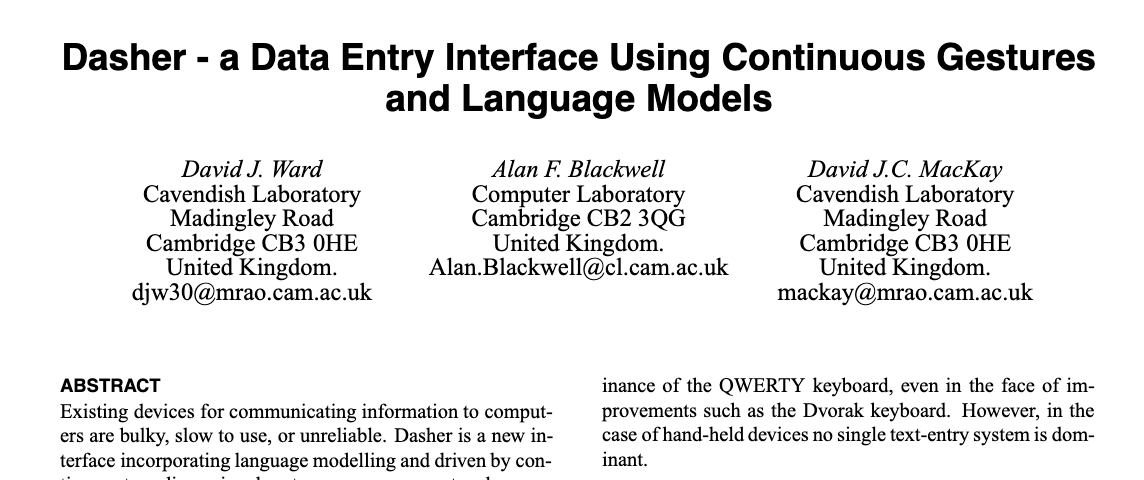
Figure: The Dasher system (Ward et al., 2000) is a pointer based text entry system that gave a very practical demonstration of the power of probability.
Figure: Dasher is a single-mode text interface designed for use with a pointer. It also contains a language model and builds on arithmetic coding to suggest the next letter.
It had multiple extensions including a breath system which David later demonstrated in Sheffield in a workshop in 2004.
One aspect that left an impression was the use of entropy to demonstrate communication rates.
Figure: The Dasher system (Ward et al., 2000) is a pointer based text entry system that gave a very practical demonstration of the power of probability.
Thermalisation from Different Initial Conditions
This simulation places exactly nine billiard balls on a 3×3 grid, each coloured according to its position. The 3×3 histogram grid tracks, for each ball, the cumulative 2-D velocity distribution \((v_x, v_y)\) it has visited since the last reset.
The entropy \(H(v_x, v_y)\) for each ball is shown in the top-left of its panel. At the start, when all balls move identically, every panel shows a single bright dot near zero entropy. As elastic collisions redistribute energy the dots spread outward, tracing the Maxwell–Boltzmann circle, and entropy climbs toward its maximum.
The coloured dot in the top-right corner of each panel matches the ball’s colour on the main canvas, making it easy to follow individual balls.
Use the Display dropdown to switch between the 2D joint distribution \(p(v_x, v_y)\) (heatmap) and the two 1D marginals \(p(v_x)\) and \(p(v_y)\) overlaid as bar charts. Both marginals are expected to converge to the same symmetric distribution; the coloured bars show \(p(v_x)\) (ball colour) and the dark outline shows \(p(v_y)\). The entropy labels \(H_x\) and \(H_y\) confirm that the two components thermalise at the same rate.
Use the Initialisation dropdown to choose how the balls start:
| Option | Description |
|---|---|
| From top ↓ | All balls move downward at the same speed |
| From bottom ↑ | All balls move upward |
| From left → | All balls move rightward |
| From right ← | All balls move leftward |
| Clockwise ↻ | Each ball moves tangentially clockwise around the canvas centre |
| Counter-CW ↺ | Each ball moves tangentially counter-clockwise |
For the four directional cases all nine histograms start at the same point, yet rapidly diverge and then converge to the same circular distribution. For the propellor cases adjacent balls start with very different velocity directions — the corner and edge balls even start at nearly opposite velocities — and yet all nine panels converge to the same equilibrium blob.
Notice that this system is ergodic: in the long-run distribution of each ball’s velocity is independent of the initial conditions and identical for all balls, even though the path to equilibrium differs.
Initialisation: Display:
Figure: Nine billiard balls on a 3×3 grid. The histogram grid tracks each ball’s cumulative \((v_x, v_y)\) velocity distribution. Entropy per ball rises from near zero (single bright dot at the initial velocity) to the Maxwell–Boltzmann value as collisions thermalise the gas. Use the Initialisation dropdown to compare directional starts (all balls move the same way) with propellor starts (adjacent balls move in opposite directions): all initial conditions converge to the same equilibrium, demonstrating ergodicity.
Figure: Samples from independent Gaussian variables that represent horizontal and vertical velocities when our system is at equilibrium.
Sampling Two Dimensional Variables
Jaynes and Maximum Entropy

Figure: Ed Jaynes who developed the maximum entropy principle
Maximum Entropy Motivation
Ed Jaynes (Jaynes, 1957), proposed a foundation for statistical mechanics based on information theory. Jaynes recast that the problem of assigning probabilities in statistical mechanics as a problem of inference with incomplete information.
A central problem in statistical mechanics is assigning initial probabilities when our knowledge is incomplete. The canonical example is if we know only the average energy of a system, what probability distribution should we use? Jaynes argued that we should use the distribution that maximises entropy subject to the constraints of our knowledge.
Jaynes illustrated the approach with a simple example. If a die has been tossed many times, with an average result of 4.5 rather than the expected 3.5 for a fair die. What probability assignment \(P_n\) (\(n=1,2,...,6\)) should we make for the next toss?
We need to satisfy two constraints \[\begin{align} \sum_{n=1}^6 P_n &= 1 \\ \sum_{n=1}^6 n P_n &= 4.5 \end{align}\]
Many distributions could satisfy these constraints, but which one makes the fewest unwarranted assumptions? Jaynes argued that we should choose the distribution that is maximally noncommittal with respect to missing information - the one that maximises the entropy, \[\begin{align} S_I = -\sum_{i} p_i \log p_i \end{align}\] This principle leads to the exponential family of distributions, which in statistical mechanics gives us the canonical ensemble and other familiar distributions.
Die Roll Simulation
This simulation illustrates the maximum entropy principle through Jaynes’ dice example (Jaynes, 1957). A fair die has expected outcome 3.5; the Jaynes example asks: if we know only that the average outcome is 4.5, what probability distribution \(P_n\) over the six faces should we assign?
The answer is the maximum-entropy distribution subject to the constraint \(\sum_{n=1}^6 n P_n = 4.5\), which belongs to the exponential family: \[\begin{align} P_n = \frac{e^{\lambda n}}{Z(\lambda)}, \qquad Z(\lambda) = \sum_{n=1}^6 e^{\lambda n} \end{align}\] where \(\lambda > 0\) is chosen so the mean constraint is satisfied. This avoids any unwarranted assumption beyond the available data.
Rolls: 0
Sample mean: —
H(p): —
Outcome weights (auto-normalised to probabilities)
Figure: Interactive die-roll simulation. Click the die or press Roll to sample from the configured distribution. The histogram shows empirical relative frequencies (coloured bars) overlaid on the theoretical probabilities (dashed outlines). Use the sliders to set arbitrary outcome weights, or click a preset to load the uniform distribution (mean 3.5), the Jaynes maximum-entropy distribution (mean 4.5), or a low-biased distribution (mean 2).
The General Maximum-Entropy Formalism
For a more general case, suppose a quantity \(x\) can take values \((x_1, x_2, \ldots, x_n)\) and we know the average values of several functions \(f_k(x)\). The problem is to find the probability assignment \(p_i = p(x_i)\) that satisfies \[\begin{align} \sum_{i=1}^n p_i &= 1 \\ \sum_{i=1}^n p_i f_k(x_i) &= \langle f_k(x) \rangle = F_k \quad k=1,2,\ldots,m \end{align}\] and maximises the entropy \(S_I = -\sum_{i=1}^n p_i \log p_i\).
Using Lagrange multipliers, the solution is the generalised canonical distribution, \[\begin{align} p_i = \frac{\exp(-\lambda_1 f_1(x_i) - \ldots - \lambda_m f_m(x_i))}{Z(\lambda_1,\ldots,\lambda_m)} \end{align}\] where \(Z(\lambda_1,\ldots,\lambda_m)\) is the partition function, \[\begin{align} Z(\lambda_1,\ldots,\lambda_m) = \sum_{i=1}^n \exp(-\lambda_1 f_1(x_i) - \ldots - \lambda_m f_m(x_i)) \end{align}\] The Lagrange multipliers \(\lambda_k\) are determined by the constraints, \[\begin{align} \langle f_k \rangle = -\frac{\partial}{\partial \lambda_k}\log Z(\lambda_1,\ldots,\lambda_m) \quad k=1,2,\ldots,m. \end{align}\] The maximum attainable entropy is \[\begin{align} (S_I)_{max} = \log Z + \sum_{k=1}^m \lambda_k \langle f_k \rangle. \end{align}\]
\[ p_i = \frac{\exp(-\lambda_1 f_1(x_i) - \ldots - \lambda_m f_m(x_i))}{Z(\lambda_1,\ldots,\lambda_m)} \] \[ Z(\ldots) = \sum_{i=1}^n \exp(-\lambda_1 f_1(x_i) - \ldots - \lambda_m f_m(x_i)) \] \[ \langle f_k \rangle = -\frac{\partial}{\partial \lambda_k}\log Z(\lambda_1,\ldots,\lambda_m) \quad k=1,2,\ldots,m. \]
Exponential Family
This mirrors a broadly used representation in statistics known as the exponential family.
\[ p(X|\boldsymbol{\theta}) = \exp\left(\sum_i \theta_i T(X) - \phi(\boldsymbol{\theta}_i)\right) \] where \(\theta_i = \lambda_i\)
Waterhouse, MacKay and Robinson
For me, I first saw this form of variational optimisation through Waterhouse et al. (n.d.) work on Bayesian Mixtures of Experts.
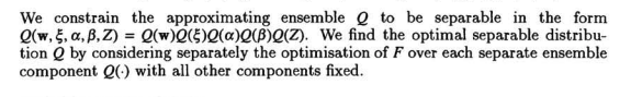
Figure: Paragraph from Waterhouse et al. (n.d.) just after equation (10) introducing a separable (mean-field) approximation to the full Bayesian posterior and the independent optimisation of each component.
This approach became a mainstay of the variational Bayesian approach to machine learning.
Figure: Two independent Gaussians for the \(x\) and \(y\) velocity of a ball.
The Classical Observer
Figure: Here the observer is monitoring the movements of the particles. We’ve plotted the velocities alongside the 1 standard deviation contour of their theoretical distribution.
The Classical Observer - Correlated
The Classical Observer - Anti-correlated
Back to self adjudication
The No-Barber Principle
In 1901 Bertrand Russell introduced a paradox: if a barber shaves everyone in the village who does not shave themselves, does the barber shave themselves? The paradox arises when a definition quantifies over a totality that includes the defining rule itself.
We propose a similar constraint for the inaccessible game: the foundational rules must not refer to anything outside themselves for adjudication or reference. Or in other words there can be no external structure. We call this the “no-barber principle.”
The no-barber principle says that admissible rules must be internally adjudicable: they depend only on quantities definable from within the system’s internal language, without requiring e.g. an external observer to define the co-ordinates or a privileged decomposition.
The Classical Observer - Inaccessible
Figure: Here the observer is blocked from monitoring anything inside the sytem.
When we don’t know what’s going on inside, we can’t express outcomes in the way we could with an observer. But we can still express entropies. This highlights an interesting characteristic of entropies. If we don’t express the probability directly, but just work with the entropies themselves, it feels like we can assess the bounds of possibility without directly expressing what’s going on.
Entropy and Impossibility
While we don’t see the underlying probability, we can capture a class of different distirbutions by considering the mapping to the system entropy.
Think of entropy as a scoring system: every probability distribution gets a number measuring its uncertainty. Once you have that, you can line them up from least to most uncertain — which gives you a natural ordering.2
We denote marginal entropy of the \(i\)th variable by \(h_i\). We denote the joint entropy of the entire system by \(H\).
Energy
Energy Constraints
The Conservation Law
The \(I + H = C\) Structure
We have established four axioms, with the fourth axiom stating that the sum of marginal entropies is conserved, \[ \sum_{i=1}^N h_i = C. \] This conservation law is the heart of The Inaccessible Game, but to understand its dynamical implications, we need to rewrite it in a more revealing form.
Multi-Information: Measuring Correlation
The multi-information (or total correlation), introduced by Watanabe (1960), measures how much the variables in a system are correlated. It is defined as, \[ I = \sum_{i=1}^N h_i - H, \] where \(H\) is the joint entropy of the full system: \[ H = -\sum_{\mathbf{x}} p(\mathbf{x}) \log p(\mathbf{x}). \]
The multi-information has a nice interpretation:
- \(I = 0\): The variables are completely independent. The joint entropy equals the sum of marginal entropies.
- \(I > 0\): The variables are correlated. Some information is “shared” between variables, so the joint entropy is less than the sum of marginals.
- \(I\) is maximal: The variables are maximally correlated (in the extreme case, deterministically related).
Multi-information is always non-negative (\(I \geq 0\)) and measures how much knowing one variable tells you about others.
Using the definition of multi-information, we can rewrite our conservation law. From \(I = \sum_{i=1}^N h_i - H\), we have: \[ \sum_{i=1}^N h_i = I + H. \] Therefore, the fourth axiom \(\sum_{i=1}^N h_i = C\) becomes: \[ I + H = C. \]
This is an information action principle. It says that multi-information plus joint entropy is conserved. This equation sits behind the dynamics of the Inaccessible Game.
This equation has the structure of an action principle in classical mechanics. In physics, total energy is conserved and splits into two parts, \[ T + V = E, \] where \(T\) is kinetic energy and \(V\) is potential energy.
The analogy for The Inaccessible Game is.
- Multi-information \(I\) plays the role of potential energy. It represents “stored” correlation structure. High \(I\) means variables are tightly coupled, like a compressed spring.
- Joint entropy \(H\) plays the role of kinetic energy. It represents “dispersed” or “free” information. High \(H\) means the probability distribution is spread out, with maximal uncertainty.
Just as a classical system evolves from high potential energy to high kinetic energy (a ball rolling down a hill), the idea in the Inaccessible Game will be that the information system evolves from high correlation (high \(I\)) to high entropy (high \(H\)).
Information Relaxation
The \(I + H = C\) structure suggests a relaxation principle: systems naturally evolve from states of high correlation (high \(I\), low \(H\)) toward states of low correlation (low \(I\), high \(H\)).
Why? Our inspiration is that the second law of thermodynamics tells us that entropy increases. If we want to introduce dynamics in the game, increasing entropy provides an obvious way to do that. Since \(I + H = C\) is constant, if \(H\) increases, \(I\) must decrease. The system breaks down correlations to increase entropy.
This is analogous to how physical systems relax from non-equilibrium states (low \(T\), high \(V\)) to equilibrium (high \(T\), low \(V\)). A compressed spring releases its stored energy. A hot object in a cold room disperses its energy. In information systems, correlated structure dissipates into entropy.
Consider a simple two-variable system with binary variables \(X_1\) and \(X_2\):
High correlation state (high \(I\), low \(H\)): \[ p(X_1=0, X_2=0) = 0.5, \quad p(X_1=1, X_2=1) = 0.5 \] The variables are perfectly correlated. Marginal entropies: \(h_1 = h_2 = 1\) bit. Joint entropy: \(H = 1\) bit. Multi-information: \(I = 1 + 1 - 1 = 1\) bit.
Low correlation state (low \(I\), high \(H\)): \[ p(X_1, X_2) = 0.25 \text{ for all four combinations} \] The variables are independent. Marginal entropies: \(h_1 = h_2 = 1\) bit. Joint entropy: \(H = 2\) bits. Multi-information: \(I = 1 + 1 - 2 = 0\) bits.
The system relaxes from the first state to the second, conserving \(I + H = 2\) bits throughout. Let’s visualise this relaxation:
import numpy as np# Generate relaxation trajectory
n_steps = 100
alphas = np.linspace(0, 1, n_steps)
h1_vals = []
h2_vals = []
H_vals = []
I_vals = []
for alpha in alphas:
p00, p01, p10, p11 = relaxation_path(alpha)
h1, h2, H, I = compute_binary_entropies(p00, p01, p10, p11)
h1_vals.append(h1)
h2_vals.append(h2)
H_vals.append(H)
I_vals.append(I)
h1_vals = np.array(h1_vals)
h2_vals = np.array(h2_vals)
H_vals = np.array(H_vals)
I_vals = np.array(I_vals)
C_vals = I_vals + H_vals # Should be constantFigure: Left: Multi-information \(I\) decreases as joint entropy \(H\) increases, conserving \(I + H = C\). The colored regions show how the conserved quantity splits between correlation (red) and entropy (blue). Right: Marginal entropies remain constant throughout, making the system inaccessible to external observation.
The visualisation shows the trade-off: as the system relaxes, correlation structure (multi-information) is converted into entropy. The total \(I + H = C\) remains constant (black dashed line), but the system evolves from a state dominated by correlation to one dominated by entropy.
The marginal entropies \(h_1\) and \(h_2\) stay constant throughout this evolution. An external observer measuring only marginal entropies would see no change—the system is informationally isolated, hence “inaccessible.”
Long Story Short
Building on these ideas, some interesting conclusions emerge. The marginal engropy constraint leads to GENERIC-like dynamics Öttinger (2005).
When characterising the origin of the game, a shift is forced from Shannon entropy to von Neumann entropy (Neumann, 1932). In retrospect the shift feels natural if we take an algebraic view of quantum probability, where outcomes are no longer primitive. This is consistent with the inaccessible nature of the game.
The game is inspired by the nice connections between inference and thermodynamics explored by E. T. Jaynes, but the dynamics play out through the framework of information geometry (Amari and Nagaoka, 2000) which makes much of the (normally complicated) calculations around Riemanian geometry relatively straightforward.
Energy

Figure: David’s book MacKay (2008) brought his clarity of thought to the challenge of sustainable energy.
Pendulum Animation
import numpy as np# Simple pendulum: trading potential ↔ kinetic energy
# State: angle θ and angular velocity ω
# Energy: E = (1/2)mL²ω² + mgL(1-cos(θ))
# Parameters
g = 9.81 # gravity
L = 1.0 # length
m = 1.0 # mass
# Initial conditions: release from angle, zero velocity
theta0 = np.pi/3 # 60 degrees
omega0 = 0.0
initial_state = np.array([theta0, omega0])
initial_energy = pendulum_energy(theta0, omega0)
# Simulate using Störmer-Verlet method (symplectic integrator, preserves energy)
dt = 0.02
t_max = 5.0
num_steps = int(t_max / dt)
# Arrays to store trajectory
times = np.linspace(0, t_max, num_steps)
trajectory = np.zeros((num_steps, 2))
energies = np.zeros(num_steps)
# Integrate using Störmer-Verlet (symplectic, time-reversible)
# Half-step omega, full-step theta, half-step omega — preserves energy to machine precision
theta, omega = initial_state
for i in range(num_steps):
trajectory[i] = [theta, omega]
energies[i] = pendulum_energy(theta, omega)
omega_half = omega - 0.5 * (g/L) * np.sin(theta) * dt
theta = theta + omega_half * dt
omega = omega_half - 0.5 * (g/L) * np.sin(theta) * dt
# Verify energy conservation
energy_drift = np.abs(energies - initial_energy).max()
print(f"Maximum energy drift: {energy_drift/initial_energy*100:.2f}%")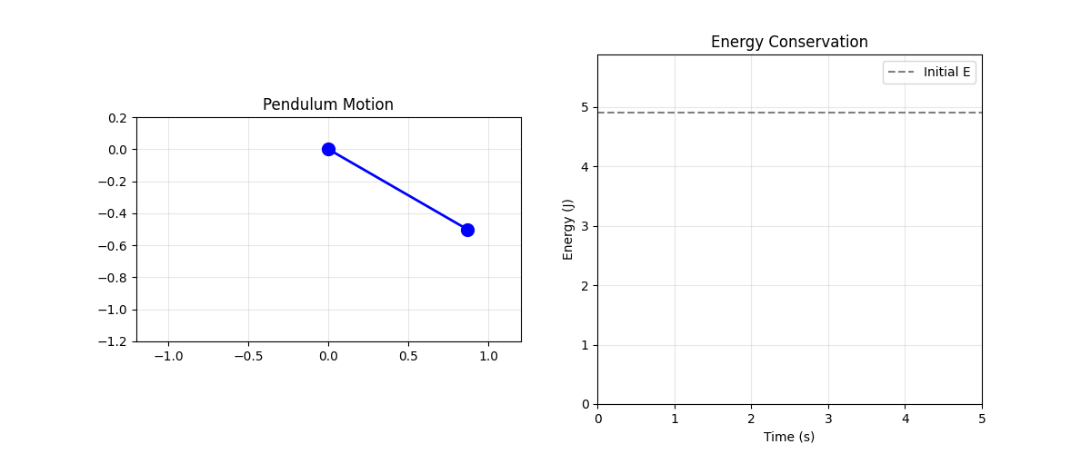
Figure: Pendulum energy conservation: the pendulum (left) trades potential and kinetic energy while total energy (red line, right) remains constant. Green shows kinetic energy, orange shows potential energy.
This pendulum simulation uses.
Energy formula: \(E = \frac{1}{2}mL^2\omega^2 + mgL(1-\cos\theta)\) (kinetic + potential)
Dynamics from energy: The equation \(\frac{\text{d}\omega}{\text{d}t} = -\frac{g}{L}\sin\theta\) comes from energy conservation structure
Trading energy: Watch kinetic (green) and potential (orange) trade off while total (red) stays constant
Geometric structure: The antisymmetric structure we’ll study ensures this conservation automatically
Störmer-Verlet integrator: The simulation uses a symplectic, time-reversible integrator — each step splits the velocity update into two half-steps either side of the position update, preserving the Hamiltonian structure and keeping energy drift at machine precision level.
The animation shows the pendulum swinging with the energy plot demonstrating near-perfect conservation.
One of the nice results of Lawrence (2025) is that in certain thermodynamic limits marginal entropy conservation manifests as energy conservation. So in these (meta-stable) regions one can use Jaynes’ maximum entropy approach to determin the stationary distribution.
Intelligence
Perpetual Motion and Superintelligence
Imagine in 1925 a world where the automobile is already transforming society, but big promises are being made for things to come. The stock market is soaring, the 1918 pandemic is forgotten. And every major automobile manufacturer is investing heavily on the promise they will each be the first to produce a car that needs no fuel. A perpetual motion machine.
Well, of course that didn’t happen. But I sometimes wonder if what we’re seeing today 100 years later is the modern equivalent of that. In 2025 billions are being invested in promises of superintelligence and artificial general intelligence that will transform everything.
We know why perpetual motion is impossible: the second law of thermodynamics tells us that entropy always increases. So we can’t have motion without entropy production. No matter how clever the design, you cannot extract energy from nothing, and you cannot create a closed system that does useful work indefinitely without an external energy source.
How might we make an equivalent statement for the bizarre claims around superintelligence? Some inspiration comes from Maxwell’s demon, an “intelligent” entity which operates against the laws of thermodynamics. The inspiration comes because the demon suggests that for the second law to hold there must be a relationship between the demon’s decisions and thermodynamic entropy.
One of the resolutions comes from Landauer’s principle, the notion that erasure of information requires heat dissipation. This suggests there are fundamental information-theoretic constraints on intelligent systems, just as there are thermodynamic constraints on engines.
I’ve no doubt that AI technologies will transform our world just as much as the automobile has. But I also have no doubt that the promise of superintelligence is just as silly as the promise of perpetual motion. The inaccessible game provides one way of understanding why.
Information-Theoretic Limits
The hope is that this framework might reveal limits on information processing systems, including intelligent systems.
Information-Theoretic Limits on Intelligence
Just as the second law of thermodynamics places fundamental limits on mechanical engines, no matter how cleverly designed, the idea is that information theory places fundamental limits on information engines, no matter how cleverly implemented.
What Intelligent Systems Must Do
Any intelligent system, whether biological or artificial, must perform certain fundamental operations:
- Acquire information from its environment (sensing, observation)
- Store information about the world (memory)
- Process information to make decisions (computation)
- Erase information to make room for new data (memory management)
- Act on the world using the processed information
Each of these operations has information-theoretic costs that cannot be eliminated by clever engineering.
Landauer’s Principle
Landauer’s principle (Landauer, 1961) establishes that erasing one bit of information requires dissipating at least \(k_BT\log 2\) of energy as heat, where \(k_B\) is Boltzmann’s constant and \(T\) is temperature.
This isn’t an engineering limitation, it’s a fundamental consequence of the second law. To reset a bit to a standard state (say, always 0) requires reducing its entropy from 1 bit to 0 bits. That entropy must go somewhere, and it ends up as heat in the environment.
This doesn’t mean AI can’t be powerful or transformative — internal combustion engines transformed the world despite thermodynamic limits. But it does mean there are hard bounds on what’s possible, and claims that ignore these bounds are as unrealistic as promises of perpetual motion.
The perpetual motion analogy provides an accessible way to think about claims of unbounded intelligence.
David’s Approach
David MacKay taught us to ask: “What are the fundamental constraints? What do the numbers actually say?” Today this way of thinking still inspires me, and the inaccessible game is the work I’m interested in that I think comes closest in spirit to that legacy.
Conclusions and Inspiration
We have explored what emerges when we demand internal adjudicability in an information-theoretic dynamical system. Starting from consistency requirements rather than physical assumptions, we derived:
Thanks!
For more information on these subjects and more you might want to check the following resources.
- company: Trent AI
- book: The Atomic Human
- twitter: @lawrennd
- podcast: The Talking Machines
- newspaper: Guardian Profile Page
- blog: http://inverseprobability.com
References
Have a look at the wonderful tributes to him on the Cambridge Ultimate website.↩︎
More formally entropy defines a functor from the category of finite probability spaces to the poset category \((\Re, \leq)\), assigning to each object its Shannon entropy.↩︎